Processing satellite images (or other remote sensing data) is a computational challenge for two reasons: normally, the images are big (many megabytes or gigabytes) and many images are needed in combination to produce the desired information.
Opening and processing many big images can consume a lot of computer memory. This condition sets a tight limit on what the user can do before running out of memory.
In this chapter, we will focus on how to perform sustainable image processing and how to open and make calculations with many big images while keeping the memory consumption low with efficient code.
The following topics will be covered:
- An introduction to satellite images and Landsat 8 data
- How to select and download Landsat 8 data
- What happens to the computer memory when we work with images?
- How to read images in chunks
- What are Python iterators and generators?
- How to iterate through an image
- How to create color compositions with the new techniques
Satellite images are a form of remote sensing data. They are composed of the information collected by satellites and are made available to users as image files. Just like the digital elevation model that we worked on before, these images are made of pixels, each one representing the value of a given attribute for a given geographic extent.
These images can be used to visualize features on Earth using real colors or they can be used to identify a variety of characteristics using parts of the light spectrum invisible to the human eyes.
In order to follow the examples, we will use images from the Landsat 8 satellite. They are available for free on the Internet. Let's take a look at some of the characteristics of this satellite.
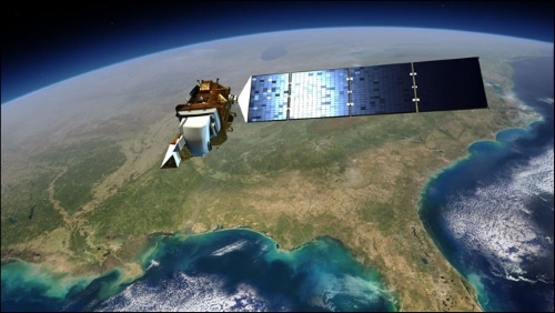
Landsat 8 carries two instruments: the Operational Land Imager (OLI) and the Thermal Infrared Sensor (TIRS).
These sensors can collect data in a total of 10 different bands processed in a resolution of 4096 possible levels (12-bit). The data is encoded into 16-bit TIFF images scaled to 55000 possible values.
|
Bands |
Wavelength (micrometers) |
Resolution (meters) |
Common uses |
|---|---|---|---|
|
Band 1—Coastal aerosol |
0.43 - 0.45 |
30 |
Shallow coastal water studies and estimation of the concentration of aerosols in the atmosphere |
|
Band 2—Blue |
0.45 - 0.51 |
30 |
Visible blue channel, distinguish soil from vegetation |
|
Band 3—Green |
0.53 - 0.59 |
30 |
Visible green channel |
|
Band 4—Red |
0.64 - 0.67 |
30 |
Visible red channel |
|
Band 5—Near Infrared (NIR) |
0.85 - 0.88 |
30 |
Biomass estimation |
|
Band 6—SWIR 1 |
1.57 - 1.65 |
30 |
Soil moisture |
|
Band 7—SWIR 2 |
2.11 - 2.29 |
30 |
Soil moisture |
|
Band 8—Panchromatic |
0.50 - 0.68 |
15 |
Sharper resolution |
|
Band 9—Cirrus |
1.36 - 1.38 |
30 |
Detection of cirrus cloud contamination |
|
Band 10—Thermal Infrared (TIRS) 1 |
10.60 - 11.19 |
30 |
Thermal mapping and estimating soil moisture |
|
Band 11—Thermal Infrared (TIRS) 2 |
11.50 - 12.51 |
30 |
Thermal mapping and estimating soil moisture |
Landsat 8 images are available freely on the Internet and there are some nice tools to find and download these images. For the book, we will use U.S Geological Survey (USGS) EarthExplorer. It's a web app packed with resources to obtain geographic data.
In order to follow the book's examples, we will download data for the same Montreal (Quebec, Canada) area that we obtained the points of interest of the previous chapter. This data is included in the book's sample data and you can skip these steps if you wish.
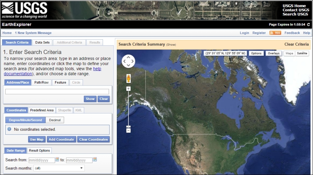
First, we will open the website and select our region of interest as follows:
- Go to the http://earthexplorer.usgs.gov/ website. You will see a map, some options at the top, and a panel with search tools on the left-hand side:
- At the top right, you will see a Login/Register button. If you don't have an account, click on Register and create a new one. Otherwise, log in to the system.
- The next step is to search for the location of interest. You can search by entering
Montrealin the box and clicking on Show. A list will appear with the search results. Click on Montreal on the list. A marker will appear and the coordinates will be set. - Click on the Data Sets button to show the available data for this coordinate.
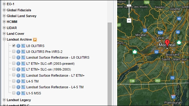
- On the next screen, expand the Landsat Archive item, select L8 OLI/TIRS, and click on the Additional Criteria button.
- Now, let's make sure that we get images with little cloud cover. Use the scroll bar to find the Cloud Cover item and select Less than 10%. Now, click on Results to see what was found.
- A new tab will open showing the results. Note that each item contains a small toolbar with a set of icons. Click on the feet icon of some of the images to see their extent on the map:
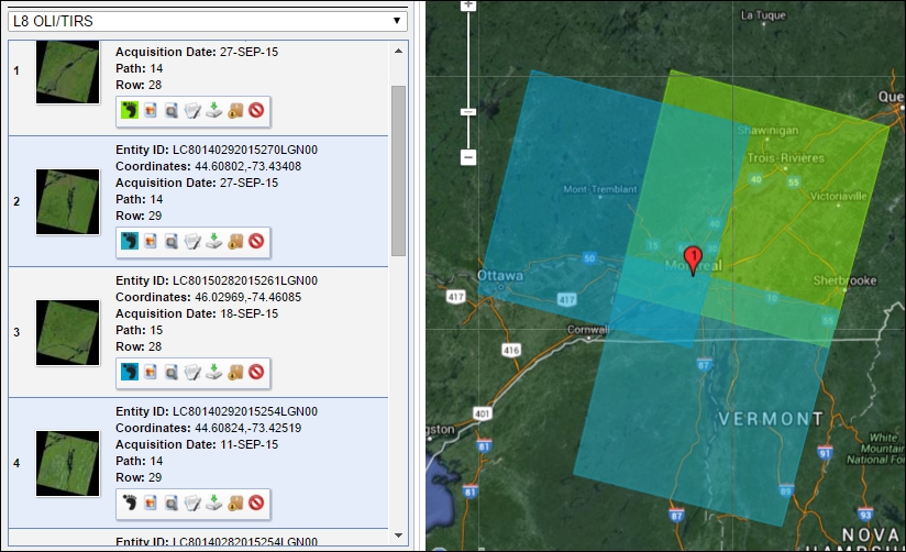
- For our examples, we need just one data set: one for path 14, row 28. Find the data for this set of rows and columns (you can use an image from any date; it's up to you) and then click on the Download Options button on the mini toolbar (it's the icon with a green arrow pointing to a hard drive).
- A window will pop up with the download options. Click on Download Level 1 GeoTIFF Data Product.
Note
USGS has an application that can manage and resume large downloads. Take a look at https://lta.cr.usgs.gov/BulkDownloadApplication for more information.
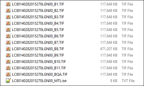
- After the download is complete, create a new folder in your
datafolder and name itlandsat. Unpack all the images in this folder.
Each package contains 12 .tif images and a text file containing the metadata. Each image name is composed of the row, column, date, and band of the image. Note that the band 8 image (B8) is much larger than the other images. This is because it has a better resolution. BQA is a quality assessment band. It contains information on the quality of each of the pixels in the image. We will see more about this band later.