Search in book...
Toggle Font Controls
Create new playlist

Name your new playlist

Playlist description (optional)
Sign In

Email address

Password

Forgot Password?

or

Continue with Facebook

Continue with Google
Sign Up

Full Name

Email address

Confirm Email Address

Password

or

Continue with Facebook

Continue with Google

Creating image compositions

Now that we know the basics of iterating through the image, which allows us to process many bands together without running out of memory, let's produce some fancier results.

True color compositions

Since we have Landsat's red, green, and blue bands, we can create an image with true colors. This means an image with colors similar to what they would be if we were directly observing the scene (for example, the grass is green and the soil is brown). To do this, we will explore a little bit more of Python's iterators.

The Landsat 8 RGB bands are respectively bands 4, 3, and 2. Following the concept that we want to automate tasks and processes, we won't repeat the commands for each one of the bands. We will program Python to do this as follows:

Edit your imports at the beginning of the file to be as follows:

import os
import cv2 as cv
import itertools
from osgeo import gdal, gdal_array
import numpy as np

Now add this new function. It will prepare the bands' paths for us:

def compose_band_path(base_path, base_name, band_number):
    return os.path.join(
        base_path, base_name) + str(band_number) + ".TIF"

To check the purpose of this function and itertools we imported, edit the if __name__ == '__main__': block with this code:

if __name__ == '__main__':
    base_path = "../../data/landsat"
    base_name = 'LC80140282015270LGN00_B'

    bands_numbers = [4, 3, 2]
    bands = itertools.imap(
        compose_band_path,
        itertools.repeat(base_path),
        itertools.repeat(base_name),
        bands_numbers)

    print(bands)
    for item in bands:
        print(item)

Now run the code and check the results:
```
<itertools.imap object at 0x02DE9510>
../../data/landsat/LC80140282015270LGN00_B4.TIF
../../data/landsat/LC80140282015270LGN00_B3.TIF
../../data/landsat/LC80140282015270LGN00_B2.TIF

Process finished with exit code 0
```
The compose band path simply joins the base path, the name of the band, and the band number in order to output a band filename with its path.
Instead of calling the function in a for loop and appending the results to a list, we used the itertools.imap function. This function takes another function as the first argument and any iterables as the other arguments. It creates an iterator that will call the function with the arguments at each iteration. The itertools.repeat function is responsible for repeating a given value infinite times when iterated.
Now, we will write the function that will combine the bands into an RGB image. Add this function to your file:
```
def create_color_composition(bands, dst_image):
    try:
        os.remove(dst_image)
    except OSError:
        pass
    # Part1
    datasets = map(gdal.Open, bands)
    img_iterators = map(create_image_generator, datasets)
    cols = datasets[0].RasterXSize
    rows = datasets[0].RasterYSize

    # Part2
    driver = gdal.GetDriverByName('GTiff')
    new_dataset = driver.Create(dst_image, cols, rows,
                                eType=gdal.GDT_Byte,
                                bands=3,
                                options=["PHOTOMETRIC=RGB"])
    gdal_array.CopyDatasetInfo(datasets[0], new_dataset)

    # Part3
    rgb_bands = map(new_dataset.GetRasterBand, [1, 2, 3])
    for index, bands_rows in enumerate(
            itertools.izip(*img_iterators)):
        for band, row in zip(rgb_bands, bands_rows):
            row = adjust_values(row, [0, 30000])
            band.WriteArray(xoff=0, yoff=index, array=row)
```
In Part 1, Python's built-in map function works like itertools.imap, but instead of an iterator, it creates a list with the results. This means that all the items are calculated and available. First, we used it to create a list of GDAL datasets by calling gdal.Open on all the bands. Then, the map function is used to create a list of image iterators, one for each band.
In Part 2, we created the output database just like we did before. But this time, we told the driver to create a dataset with three bands, each with byte data type (256 possible values). We also tell that it's an RGB photo in the options.
In Part 3, we used the map function again to get the reference to the bands in the dataset. In the first for loop, at each iteration, we got an index, that is, the row number, and a tuple containing a row for every band.
In the nested for loop, each iteration gets one of the output image bands and one row of the input bands. The values of the row are then converted from 16-bit to 8-bit (byte) with our adjust_values function. To adjust the values, we passed a magic number in order to get a brighter image. Finally, the row is written to the output band.

Finally, let's test the code. Edit your if __name__ == '__main__': block:

if __name__ == '__main__':
    base_path = "../../data/landsat/"
    base_name = 'LC80140282015270LGN00_B'

    bands_numbers = [4, 3, 2]
    bands = itertools.imap(
        compose_band_path,
        itertools.repeat(base_path),
        itertools.repeat(base_name),
        bands_numbers)

    dst_image = "../output/color_composition.tif"
    create_color_composition(bands, dst_image)

Now run it. After it's done, open the image (color_composition.tif) in the output folder. You should see this beautiful color image: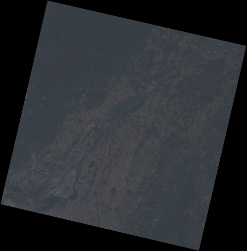

You can play with the numbers that we passed to the adjust_values function. Try changing the lower limit and the upper limit; you will get different variations of brightness.

Processing specific regions

Now, let's change our code to crop the image for us, so we can have a better view of the details of the region around Montreal. It's something like we did before. But instead of cropping the image after processing, we will only process the region of interest, making the code much more efficient.

Edit the create_image_generator function:

def create_image_generator(dataset, crop_region=None):
    if not crop_region:
        cols = dataset.RasterXSize
        rows = dataset.RasterYSize
        xoff = 0
        yoff = 0
    else:
        xoff = crop_region[0]
        yoff = crop_region[1]
        cols = crop_region[2]
        rows = crop_region[3]
    for row_index in xrange(yoff, yoff + rows):
        yield dataset.ReadAsArray(xoff=xoff, yoff=row_index,
                                  xsize=cols, ysize=1)

Now, the function receives an optional crop_region argument and only yields rows of the region of interest if it's passed. If not, it yields rows for the whole image.

Change the create_color_composition class to work with the cropped data:

def create_color_composition(bands, dst_image, crop_region=None):
    try:
        os.remove(dst_image)
    except OSError:
        pass
    datasets = map(gdal.Open, bands)
    img_iterators = list(itertools.imap(
        create_image_generator, datasets,
        itertools.repeat(crop_region)))

    if not crop_region:
        cols = datasets[0].RasterXSize
        rows = datasets[0].RasterYSize
    else:
        cols = crop_region[2]
        rows = crop_region[3]

    driver = gdal.GetDriverByName('GTiff')
    new_dataset = driver.Create(dst_image, cols, rows,
                                eType=gdal.GDT_Byte,
                                bands=3,
                                options=["PHOTOMETRIC=RGB"])
    gdal_array.CopyDatasetInfo(datasets[0], new_dataset)
    rgb_bands = map(new_dataset.GetRasterBand, [1, 2, 3])
    for index, bands_rows in enumerate(
            itertools.izip(*img_iterators)):
        for band, row in zip(rgb_bands, bands_rows):
            row = adjust_values(row, [1000, 30000])
            band.WriteArray(xoff=0, yoff=index, array=row)

Note that when img_iterators was created, we replaced the map function by itertools.imap in order to be able to use the itertools.repeat function. Since we need img_iterators to be a list of iterators, we used the list function.

Finally, edit the if __name__ == '__main__': block to pass our region of interest:

if __name__ == '__main__':
    base_path = "../../data/landsat/"
    base_name = 'LC80140282015270LGN00_B'

    bands_numbers = [4, 3, 2]
    bands = itertools.imap(
        compose_band_path,
        itertools.repeat(base_path),
        itertools.repeat(base_name),
        bands_numbers)

    dst_image = "../output/color_composition.tif"
    create_color_composition(bands, dst_image,
                             (1385, 5145, 1985, 1195))

Run the code. You should now have this nice image of Montreal:

False color compositions

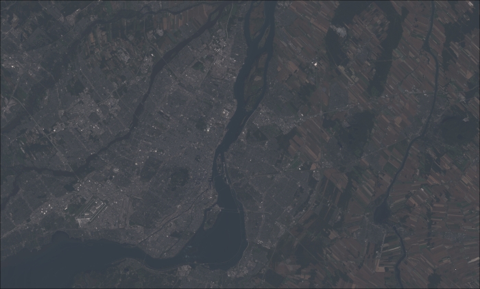
Color compositions are a great tool for information visualization, and we can use it even to see things that would be otherwise invisible to the human eye.

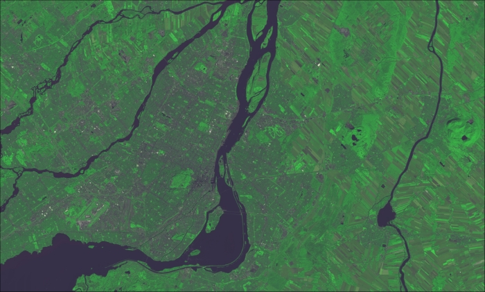
Landsat 8 and other satellites provide data in ranges of the spectrum that are reflected or absorbed more or less by specific objects. For example, vigorous vegetation reflects a lot of near-infrared radiation, so if we are looking for information on vegetation coverage or plant growth, we should consider this band.

Besides the computational analysis of different bands, we are able to visualize them by replacing the red, blue, and green components by other bands. Let's try it as follows:

Just edit the if __name__ == '__main__': block, so we use the near infrared (band 5) as the green component of the RGB image:

if __name__ == '__main__':
    base_path = "../../data/landsat/"
    base_name = 'LC80140282015270LGN00_B'

    bands_numbers = [4, 5, 2]
    bands = itertools.imap(
        compose_band_path,
        itertools.repeat(base_path),
        itertools.repeat(base_name),
        bands_numbers)

    dst_image = "../output/color_composition.tif"
    create_color_composition(bands, dst_image,
                             (1385, 5145, 1985, 1195))

Run the code and look at the output image:
You can have many other combinations. Just change the band_numbers variables to achieve different results. Try changing it to [6, 5, 2 ]. Run the code and look at how the farm fields stand out from the other features.