Satellite images come in a different format and serve different purposes. These images can be used to visualize features on Earth using real colors or they may be used to identify a variety of characteristics using parts of the spectrum invisible to the human eye.
As we saw, our sample image had three channels (blue, green, and red) that were combined in a single file to compose a real color image. Different from the sample image, most satellite data comes with each channel separated into a file for each one of them. These channels are called bands and comprise of a range of the electromagnetic spectrum visible or not to the human eye.
In the following examples, we are going to use the digital elevation models (DEM) generated with the data obtained by the Advanced Spaceborne Thermal Emission and Reflection Radiometer (ASTER).
These DEM have a resolution of approximately 90 m and the values are stored in the 16 bits signed integers representing the elevation in meters.
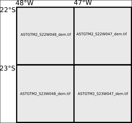
The dataset we are going to use is included in the data folder and is from a Brazilian city called Poços de Caldas. This city is inside a giant extinct volcano crater, a feature we hope to see during data processing. For didactic reasons and in order to cover a big region, four images will be used:
Note
You can obtain more digital elevation models at http://earthexplorer.usgs.gov/.
- If want to download and use your own DEM, you need to extract the downloaded ZIP file. Notice that each ZIP archive has two images. The one ending with
_demis the actual elevation data. The one ending with_numcontains the quality assessment information. Take a look at the includedREADME.pdffile for more information. - Move or copy all the images to the
datafolder of yourChapter 6code.
Each image represents a tile of 1 degree. The information on which tile the image covers is encoded in the name of the file, as seen in the following image:
Mapnik has the ability to read tiled data from the disk using the raster data source. But we are not going to use it, because the process of patching images together is very important and is worth learning.
The next code will open the images, combine them, and save a single combined image in the disk. This process (with varying levels of complexity) is called mosaicking:
- Still in the
image_experiments.pyfile, add a new function after theopen_raster_filefunction:def combine_images(input_images): """Combine images in a mosaic. :param input_images: Path to the input images. """ images = [] for item in input_images: images.append(open_raster_file(item)) print images - Now, edit the
if __name__ == '__main__':block so we can test the code:if __name__ == '__main__': elevation_data = [ '../../data/ASTGTM2_S22W048_dem.tif', '../../data/ASTGTM2_S22W047_dem.tif', '../../data/ASTGTM2_S23W048_dem.tif', '../../data/ASTGTM2_S23W047_dem.tif'] combine_images(elevation_data) - Run the code and look at the output:
[array([[[1, 1, 1],
        [1, 1, 1],
        [2, 2, 2],
        ...,
        [4, 4, 4],
        [4, 4, 4],
        [4, 4, 4]],
. . .

Process finished with exit code 0
You should see a list of four arrays. PyCharm will hide some values so it can fit in the console.
The first thing we should notice is that the order of the images in the input images argument is the same as the order of the arrays in the output list. This will be very important later.
Secondly, although the elevation data is a 16-bit signed integer (int16), the arrays representing the images still have three bands of an 8-bit unsigned integer. This is an error. OpenCV is converting the grayscale image to a color image. We are going to fix it as follows:
- Change the
open_raster_filefunction to accept a new argument. It will allow us to open the images without changing them:def open_raster_file(image, unchanged=True): """Opens a raster file. :param image: Path of the raster file or np array. :param unchanged: Set to true to keep the original format. """ flags = cv2.CV_LOAD_IMAGE_UNCHANGED if unchanged else -1 image = cv2.imread(image, flags=flags) return imageThe
flagsargument incv2.imreadallows us to tune how the images are opened and converted into arrays. If the flags are set tocv2.CV_LOAD_IMAGE_UNCHANGED, the image will open as it is without any conversion. - Since we set the default of
unchangedtotrue, we will just run the code again and see the results:[array([[ 508, 511, 514, ..., 1144, 1148, 1152], [ 507, 510, 510, ..., 1141, 1144, 1150], [ 510, 508, 506, ..., 1141, 1145, 1154], ..., [ 805, 805, 803, ..., 599, 596, 593], [ 802, 797, 803, ..., 598, 594, 590], [ 797, 797, 800, ..., 603, 596, 593]], dtype=uint16) . . . Process finished with exit code 0
The values now are correct and they are the measured elevation in meters for each pixel.
So far, we have a list of arrays in the order that the input files are listed. To figure out the next step, we can imagine this list as if the images were mosaicked as a strip:
Now, we must reorganize this, so the images are placed in their correct position. Remember that NumPy arrays have a shape property. In a 2D array, it's a tuple containing the shape in columns and rows. NumPy arrays also have the reshape() method that performs a shape transformation.
Note
Take a look at the NumPy documentation on the reshape method and function. Changing the shape of an array is a very powerful tool at http://docs.scipy.org/doc/numpy/reference/generated/numpy.reshape.html.
The reshape works by filling a row with the input values in order. When the row is full, the method jumps to the next row and continues until the end. So, if we pass the expected shape of the mosaic to the combine_images function, we can use this information to combine the images with respect to the proper positions.
But we need something else. We need to know the shape of the output image through the number of pixels, and this will be the product of the shape of each image by the shape of the mosaic. Let's try a few changes in the code as follows:
- Edit the combine images function:
def combine_images(input_images, shape, output_image):
    """Combine images in a mosaic.

    :param input_images: Path to the input images.
    :param shape: Shape of the mosaic in columns and rows.
    :param output_image: Path to the output image mosaic.
    """
    if len(input_images) != shape[0] * shape[1]:
        raise ValueError(
            "Number of images doesn't match the mosaic shape.")
    images = []
    for item in input_images:
        images.append(open_raster_file(item))
    rows = []
    for row in range(shape[0]):
        start = (row * shape[1])
        end = start + shape[1]
        rows.append(np.concatenate(images[start:end], axis=1))
    mosaic = np.concatenate(rows, axis=0)
    print(mosaic)
    print(mosaic.shape)
Now the function accepts two more arguments, the shape of the mosaic (the number of images in the row and columns and not the number of pixels) and the path of the output image for later use.
With this code, the list of images is separated into rows. Then, the rows are combined to form the complete mosaic.
- Before you run the code, don't forget to import NumPy at the beginning of the file:
# coding=utf-8 import cv2 import numpy as np And edit the if __name__ == '__main__': block: if __name__ == '__main__': elevation_data = [ '../../data/ASTGTM2_S22W048_dem.tif', '../../data/ASTGTM2_S22W047_dem.tif', '../../data/ASTGTM2_S23W048_dem.tif', '../../data/ASTGTM2_S23W047_dem.tif'] combine_images(elevation_data, shape=(2, 2)) - Now run the code and see the results:
[[508 511 514 ..., 761 761 761]
 [507 510 510 ..., 761 761 761]
 [510 508 506 ..., 761 761 761]
 ...,
 [514 520 517 ..., 751 745 739]
 [517 524 517 ..., 758 756 753]
 [509 509 510 ..., 757 759 760]]
(7202, 7202)

Process finished with exit code 0
It's now a single array with 7202 x 7202 pixels. The remaining task is to save this array to the disk as an image.
- Just add two lines to the function and edit the
if __name__ == '__main__':block:def combine_images(input_images, shape, output_image): """Combine images in a mosaic. :param input_images: Path to the input images. :param shape: Shape of the mosaic in columns and rows. :param output_image: Path to the output image mosaic. """ if len(input_images) != shape[0] * shape[1]: raise ValueError( "Number of images doesn't match the mosaic shape.") images = [] for item in input_images: images.append(open_raster_file(item)) rows = [] for row in range(shape[0]): start = (row * shape[1]) end = start + shape[1] rows.append(np.concatenate(images[start:end], axis=1)) mosaic = np.concatenate(rows, axis=0) print(mosaic) print(mosaic.shape) cv2.imwrite(output_image, mosaic) if __name__ == '__main__': elevation_data = [ '../../data/ASTGTM2_S22W048_dem.tif', '../../data/ASTGTM2_S22W047_dem.tif', '../../data/ASTGTM2_S23W048_dem.tif', '../../data/ASTGTM2_S23W047_dem.tif'] combine_images(elevation_data, shape=(2, 2), output_image="../output/mosaic.png")
If you run the previous code, you will see a black image as an output. This happens because the value range that represents the actual data of this region is so narrow in comparison to the possible range of the 16-bit integer image that we can't distinguish the shades of gray. For better understanding, let's make a simple test as follows:
- Still in the
image_experiments.pyfile, comment theif __name__ == '__main__':block and add this new one:if __name__ == '__main__': image = open_raster_file("../output/mosaic.png") print(image.min(), image.max()) - Run the code and look at the console output.
(423, 2026)

Process finished with exit code 0
Precisely, the image ranges from -32768 to 32767 and the elevation of the region in it ranges from 423 to 2026. So what we need to do to make the image visible is to scale the altitude range to the range of the data type.
Since we are making a data representation intended for human visualization, we don't need to use a big range of gray values. The researches vary, but some say that we can detect only 30 shades, so an 8-bit unsigned integer with 256 possible values should be more than enough for data visualization.
- Add this new function:
def adjust_values(input_image, output_image, img_range=None):
    """Create a visualization of the data in the input_image by
    projecting a range of values into a grayscale image.

    :param input_image: Array containing the data
     or path to an image.
    :param output_image: The image path to write the output.
    :param img_range: specified range of values or None to use the
     range of the image (minimum and maximum).
    """
    image = open_raster_file(input_image)
    if img_range:
        min = img_range[0]
        max = img_range[1]
    else:
        min = image.min()
        max = image.max()
    interval = max - min
    factor = 256.0 / interval
    output = image * factor
    cv2.imwrite(output_image, output)
This function accepts either an array or the path to an image file. With this feature, we can later use this function as a sub-step in other processing procedures. The range of values that you want to use is also optional. It can be set manually or can be extracted from the images minimum and maximum value.
- To test the code, edit the
if __name__ == '__main__':block:if __name__ == '__main__': # Adjust. adjust_values('../output/mosaic.png', '../output/mosaic_grey.png')Note that the output image is now a
pngfile. Since we are preparing the image for visualization, we can afford to lose information in data compression in exchange for a smaller file. - Run the code and open the
mosaic_grey.pngfile to see the results. You should see the following beautiful grayscale image now: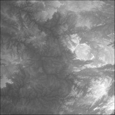
We made a big mosaic of images in order to cover the region of interest, and in the process, we ended up with an image much bigger than the one we needed. Now, it's time to crop the image, so we end up with a smaller one comprising only of what we want to see, thus saving disk space and processing time.
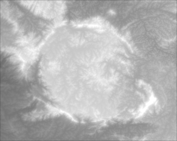
In our example, we are interested in the volcano crater. It's the round object located on the right-hand side of the image. In order to obtain only that region of interest, we will write a function that can crop the image using a bounding box set of coordinates, as follows:
- Add the new function to the
image_experiments.pyfile:def crop_image(input_image, image_extent, bbox, output_image): """Crops an image by a bounding box. bbox and image_extent format: (xmin, ymin, xmax, ymax). :param input_image: Array containing the data or path to an image. :param image_extent: The geographic extent of the image. :param output_image: The image path to write the output. :param bbox: The bounding box of the region of interest. """ input_image = open_raster_file(input_image) img_shape = input_image.shape img_geo_width = abs(image_extent[2] - image_extent[0]) img_geo_height = abs(image_extent[3] - image_extent[1]) # How much pixels are contained in one geographic unit. pixel_width = img_shape[1] / img_geo_width pixel_height = img_shape[0] / img_geo_height # Index of the pixel to cut. x_min = abs(bbox[0] - image_extent[0]) * pixel_width x_max = abs(bbox[2] - image_extent[0]) * pixel_width y_min = abs(bbox[1] - image_extent[1]) * pixel_height y_max = abs(bbox[3] - image_extent[1]) * pixel_height output = input_image[y_min:y_max, x_min:x_max] cv2.imwrite(output_image, output)Since we are dealing with NumPy arrays, the cropping itself is a simple array slicing. The slicing of arrays is very similar to the Python lists' slicing, but with additional dimensions. The statement
input_image[y_min:y_max, x_min:x_max]tells that we want only the portion of the array contained within the specified cells (that is, pixels). So, all the math involved is to convert geographic units into array indices. - Edit the
if __name__ == '__main__':block to test the code:if __name__ == '__main__': # Crop. roi = (-46.8, -21.7, -46.3, -22.1) # Region of interest. crop_image('../output/mosaic_grey.png', (-48, -21, -46, -23), roi, "../output/cropped.png") - Run the code and open the output image to see the results.
- If you have missed any of the steps, you can run the whole process all at once. Just edit the
if __name__ == '__main__'block:if __name__ == '__main__': # Combine. elevation_data = [ '../../data/ASTGTM2_S22W048_dem.tif', '../../data/ASTGTM2_S22W047_dem.tif', '../../data/ASTGTM2_S23W048_dem.tif', '../../data/ASTGTM2_S23W047_dem.tif'] combine_images(elevation_data, shape=(2, 2), output_image="../output/mosaic.png") # Adjust. adjust_values('../output/mosaic.png', '../output/mosaic_grey.png') # Crop. roi = (-46.8, -21.7, -46.3, -22.1) # Region of interest. crop_image('../output/mosaic_grey.png', (-48, -21, -46, -23), roi, "../output/cropped.png")
Our digital elevation model image has improved a lot after we processed it, but it is still not suitable for a map. Untrained eyes may find it difficult to understand the relief only by looking at the different shades of gray.
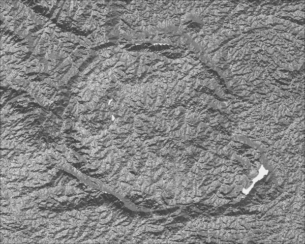
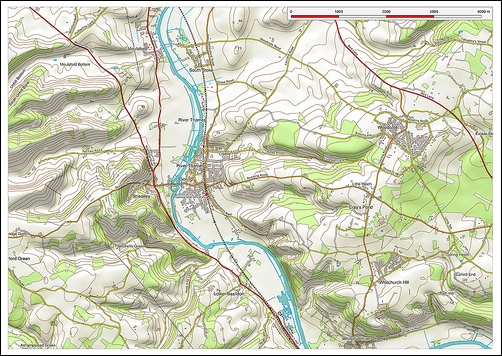
Fortunately, there is a technique, called hill shading or relief shading, that transforms the elevation data into a simulated sun shading over the terrain. Look at the beautiful map in the following picture and note how much easier it is to understand the relief when it is presented as a shaded relief:
The process is simple and involves passing our image through a well-known algorithm as follows:
- Add the
create_hillshadefunction to yourimage_experiments.pyfile:def create_hillshade(input_image, output_image, azimuth=90, angle_altitude=60): """Creates a shaded relief image from a digital elevation model. :param input_image: Array containing the data or path to an image. :param azimuth: Simulated sun azimuth. :param angle_altitude: Sun altitude angle. """ input_image = open_raster_file(input_image) x, y = np.gradient(input_image) slope = np.pi / 2 - np.arctan(np.sqrt(x * x + y * y)) aspect = np.arctan2(-x, y) az_rad = azimuth * np.pi / 180 alt_rad = angle_altitude * np.pi / 180 a = np.sin(alt_rad) * np.sin(slope) b = np.cos(alt_rad) * np.cos(slope) * np.cos(az_rad - aspect) output = 255 * (a + b + 1) / 2 cv2.imwrite(output_image, output) - Now, alter the
if __name__ == '__main__':block to test the code:if __name__ == '__main__': create_hillshade("../output/cropped.png", "../output/hillshade.png") - Run the code and open the output image to see the results. If everything goes fine, you should see a shaded relief representation of your data.