
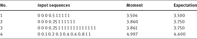
Compared to the moment-preserving technique, the approach based on the expectation of first-order derivatives can solve the problem of multiresponse (misdetection of several edges). One comparison of these two techniques is given in Table 2.3. For some similar sequences, the subpixel-level location for the expectation technique is less sensitive to the length of the input sequence.
Using Tangent Direction Information: Both of the above methods detect the subpixel-level edges using the statistical property of the blurred boundary that has a certain width, so the edge location can be determined using the information along the normal direction to the boundary. In cases where the boundary ramp is sharp, there would be few boundary pixels used for the statistical computation, and then, the error in determining the boundary would be larger. If the shape of the object is given, then the following technique can be used, which is based on the information along the tangent direction (Zhang, 2001c). Such a technique can be split into two steps: The detection of the boundary at the pixel level and then the adjustment, according to information along the tangent direction at the pixel-level boundary, of the edge location at the subpixel level. The first step could be a normal edge detection step. Only the second step is discussed in the following.
Consider Figure 2.17, in which the edge to be located is at the boundary of a circle. Let the function of this circle be (x – xc)2 + (y – yc)2 = r2, where the center coordinates are (xc, yc) and the radius is r. If the boundary points along the X- and Y-axes can be found, then both (xc, yc) and r can be obtained, and the circle can be determined.
Figure 2.17 illustrates the principle used to find the left point along the X-axis. The pixels located inside the circle are shaded. Let x1 be the coordinate of the left-most point along the X direction and h be the number of boundary pixels in the column with X coordinate x1. At this column, the difference T between two cross-points that are produced by two adjacent pixels with the real circle is
Suppose S is the difference between the coordinate xl and the real subpixel edge. In other words, S is needed to modify the pixel-level boundary to the subpixel-level boundary. It is easy to see from Figure 2.17 that S is the summation of all T(i) for i = 1, 2, ..., h and pluse
where e ∈ [0, T(h + 1)], whose average is T(h + 1)/2. Calculating T(h +1) from eq. (2.23) and putting the result into eq. (2.24) finally gives

There will be two kinds of errors when using S to modify the pixel-level boundary to produce the subpixel-level boundary. One error comes from the averaging of e, called |dSe|. The maximal of this error is
From Figure 2.17 and with the help of eq. (2.24), it can obtain
Expand the right side of eq. (2.27) and put the result into eq. (2.26), then eq. (2.26) becomes
Another error comes from the truncation. In the above, r is assumed to be the real radius. However, in a real situation, r can only be obtained in the first step with pixel-level accuracy. Suppose the variation of S caused by r is |dSr|. Apply the derivation of eq. (2.25) to r, it has
Simplifying eq. (2.29) with the help of eq. (2.27) yields (the average of dr is 0.5 pixel)
The overall error would be the sum of |dSe| and |dSr|, where the first term is the main part.
2.3.2.2Generalization of the Hough Transform
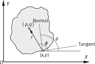
The generalization of the Hough transform could solve the problem that the object has no simple analytic form but has a particular silhouette (Ballard, 1982). Suppose for a moment that the object appears in the image with a known shape, orientation, and scale. Now pick a reference point (p, q) in the silhouette and draw a line to the boundary. At the boundary point (x, y), compute the gradient angle θ (the angle between the normal at this point and the x-axis). The radius that connects the boundary point (x, y) to the reference point (p, q) is denoted r, the angle between this connection and the x-axis (vector angle) is ϕ. Both r and ϕ are functions of θ. Thus, it is possible to precompute the location of the reference point from boundary points (when the gradient angle is given) by
The set of all such locations, indexed by the gradient angles, comprises a table called the R-table. Figure 2.18 shows the relevant geometry and Table 2.4 shows the form of the R-table.
From the above table, it can be seen that all possible reference points can be determined given a particular θ. The R-table provides a function that connects the gradient angle θ and the coordinates of a possible reference point. The following process would be similar to the normal Hough transform.
A complete Hough transform should consider, besides translation, also the scaling and rotation. Taking all these possible variations of the boundary, the parameter space would be a 4-D space. Here, the two added parameters are the orientation parameter β (the angle between the X-axis and the major direction of the boundary) and the scaling parameter S. In this case, the accumulative array should be extended to A(pmin : pmax, qmin: qmax, βmin : βmax, Smin: Smax). Furthermore, eqs. (2.31) and (2.32) should be extended to eqs. (2.33) and (2.34), respectively
2.4Segmentation Evaluation
One important fact in the development of segmentation techniques is that no general theory exists, so this development has traditionally been an ad hoc (made for a particular purpose) and problem-oriented process. As a result, all the developed segmentation techniques are generally application dependent. On the other hand, given a particular application, developing an appropriate segmentation algorithm is still quite a problem. Segmentation evaluation is thus an important task in segmentation research.
2.4.1A Survey on Evaluation Methods
Many efforts have been put into segmentation evaluation and many methods have been proposed. An overview is provided below.
2.4.1.1Classification of Evaluation Methods
Segmentation algorithms can be evaluated analytically or empirically. Accordingly, evaluation methods can be divided into two categories: analytical methods and empirical methods. The analytical methods directly examine and assess the segmentation algorithms themselves by analyzing their principles and properties. The empirical methods indirectly judge the segmentation algorithms by applying them to test images and measuring the quality of segmentation results. Various empirical methods have been proposed. Most of them can still be classified into two categories: The empirical goodness methods and the empirical discrepancy methods. In the first category, some desirable properties of segmented images, often established according to human intuition, are measured by “goodness” parameters. The performances of segmentation algorithms under investigation are judged by the values of the goodness measurements. In the second category, some references that present the ideal or expected segmentation results are found first. The actual segmentation results obtained by applying a segmentation algorithm, which is often preceded by preprocessing and/or followed by postprocessing processes, are compared to the references by counting their differences. The performances of segmentation algorithms under investigation are then assessed according to the discrepancy measurements. Following this discussion, three groups of methods can be distinguished.
A recent study on image segmentation evaluation (Zhang, 2015c) shows that most recent works are focused on the discrepancy group, while few works rely on the goodness group.
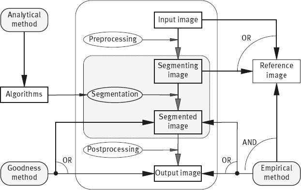
The above classification of evaluation methods can be seen more clearly in Figure 2.19, where a general scheme for segmentation and its evaluation is presented (Zhang, 1996c). The input image obtained by sensing is first (optionally) preprocessed to produce the segmenting image for the segmentation (in its strict sense) procedure. The segmented image can then be (optionally) postprocessed to produce the output image. Further processes such as feature extraction and measurement are done based on these output images.
In Figure 2.19, the part enclosed by the rounded square with the dash-dot line corresponds to the segmentation procedure in its narrow sense, while the part enclosed by the rounded square with the dot line corresponds to the segmentation procedure in its general form. The black arrows indicate the processing directions of the segmentation. The access points for the three groups of evaluation methods are depicted with gray arrows in Figure 2.19. Note that there is an OR condition between both arrows leading to the boxes containing the “segmented image” and the “output image” both from the “empirical goodness method” and the “empirical discrepancy method.” Moreover, there is an AND condition between the arrow from the “empirical discrepancy method” to the “reference image” and the two (OR-ed) arrows going to the “segmented image” and the “output image.” The analysis methods are applied to the algorithms for segmentation directly. The empirical goodness methods judge the segmented image or the output image to indirectly assess the performance of algorithms. For applying empirical discrepancy methods, the reference image is necessary. It can be obtained manually or automatically from the input image or the segmenting image. The empirical discrepancy methods compare the segmented image or the output image with the reference image and use their differences to assess the performances of algorithms.
In the following, some basic criteria are described according to this classification (more criteria can be found in Zhang (2001b, 2006b, and 2015c)).
2.4.1.2Analytical Methods
Using the analytical methods to evaluate segmentation algorithms avoids the concrete implementation of these algorithms, and the results can be exempt from the influence caused by the arrangement of evaluation experiments as empirical methods do. However, not all properties of segmentation algorithms can be obtained by analytical studies. Two examples are shown as follows:
A Priori Knowledge: Such knowledge for certain segmentation algorithms is ready to be analyzed, which is mainly determined by the nature of the algorithms. However, such knowledge is usually heuristic information, and different kinds of a priori knowledge are hardly comparable. The information provided by this method is then rough and qualitative. On the other hand, not only “the amount of the relevant a priori knowledge that can be incorporated into the segmentation algorithm is decisive for the reliability of the segmentation methods,” but it is also very important for the performance of the algorithm to know how such a priori knowledge has been incorporated into the algorithm (Zhang, 1991b).
Detection Probability Ratio: The analytical methods in certain cases can provide quantitative information about segmentation algorithms. Let T be the edge decision threshold, Pc be the probability of correct detection, and Pf be the probability of false detection. It can be derived that
The plot of Pc versus Pf in terms of T can provide a performance index of the detectors, which is called the detection probability ratio. Such an index is useful for evaluating the segmentation algorithms based on edge detection (Abdou, 1979).
2.4.1.3Empirical Goodness Methods
The methods in this group evaluate the performance of algorithms by judging the quality of the segmented images. To do this, certain quality measurements should be defined. Most measurements are established according to human intuition about what conditions should be satisfied by an “ideal” segmentation (e. g., a pretty picture). In other words, the quality of segmented images is assessed by some “goodness” measurement. These methods characterize different segmentation algorithms by simply computing the goodness measurements based on the segmented image without the a priori knowledge of the correct segmentation. The application of these evaluation methods exempts the requirement for references so that they can be used for on-line evaluation. Different types of goodness measurements have been proposed.
Goodness Based on intra-region Uniformity: It is believed that an adequate segmentation should produce images having higher intra-region uniformity, which is related to the similarity of the property about the region element (Nazif, 1984). The uniformity of a feature over a region can be computed based on the variance of that feature evaluated at every pixel belonging to that region. In particular, for a gray-level image f(x, y), let Ri be the ith segmented region and Ai be the area of Ri. The gray-level uniformity measure (GU) of f(x, y) is given by
Goodness Based on Inter-region Contrast: It is also believed that an adequate segmentation should in addition produce images having higher contrast across adjacent regions. In a simple case where a gray-level image f(x, y) consists of the object with an average gray-level fo and the background with an average gray-level fb, a gray-level inter-region contrast measure (GC) can be computed by
2.4.1.4Empirical Discrepancy Methods
In practical segmentation applications, some errors in the segmented image can be tolerated. On the other hand, if the segmenting image is complex and the algorithm used is fully automatic, the error is inevitable. The disparity between an actual segmented image and a correctly/ideally segmented image (reference image) can be used to assess the performance of algorithms. Both the actually segmented and the reference images are obtained from the same input image. The reference image is sometimes called a gold standard. A higher value of the discrepancy measurement would imply a bigger error in the actually segmented image relative to the reference image and this indicates the poorer performance of the applied segmentation algorithms.
Discrepancy Based on the Number of Misclassified Pixels: Considering the image segmentation as a pixel classification process, the percentage or the number of pixels misclassified is the discrepancy measurement that comes most readily to mind. One of them is called the probability of error(PE). For a two-class problem the PE can be calculated by
where P(B|O) is the probability of the error when classifying objects as the background, P(O|B) is the probability of the error when classifying the background as objects, P(O) and P(B) are a priori probabilities of the objects and the background in images. For the multi-class problem, a general definition of PE can be found.
Discrepancy Based on the Position of Misclassified Pixels: The discrepancy measurements based only on the number of misclassified pixels do not take into account the spatial information of these pixels. It is thus possible that images segmented differently can have the same discrepancy measurement values if these measurements only count the number of misclassified pixels. To address this problem, some discrepancy measurements based on position of mis-segmented pixels have been proposed.
One solution is to use the distance between the misclassified pixel and the nearest pixel that actually belongs to the misclassified class. Let N be the number of misclassified pixels for the whole image and d(i) be a distance metric from the ith misclassified pixel to the nearest pixel that actually is of the misclassified class. A discrepancy measurement(D) based on this distance is defined by Yasnoff (1977)
In eq. (2.4), each distance is squared. This measurement is further normalized (ND) to exempt the influence of the image size and to give it a suitable value range by Yasnoff (1977)
where A is the total number of pixels in the image (i. e., a measurement of area).
2.4.2An Effective Evaluation Method
An effective approach for the objective and quantitative evaluation and comparison of segmentation algorithms is as follows (Zhang, 1994; 1998b).
2.4.2.1Primary Conditions and General Framework
As is made evident from the discussions presented above, the following conditions should be satisfied for an evaluation and comparison procedure.
1.It should be general, that is., be suitable for all segmentation techniques and various applications. This implies that no parameters or properties of particular segmentation algorithms can be involved so that no bias with respect to some special techniques is introduced.
2.It should use quantitative and objective criteria for performance assessment. Here, quantitative means exactness (Zhang, 1997b), while objective refers to the segmentation goal and reality.
3.It should use images that can be reproduced by all users in different places for the purpose of algorithm testing. Moreover, these images should reflect common characteristics of real applications.
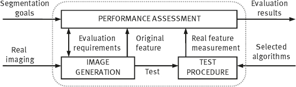
Considering these conditions, a general evaluation framework is designed. It consists of three related modules as shown in Figure 2.20. The information concerning segmentation goals, image contents, and imaging conditions can be selectively incorporated into this framework to generate the test images (Zhang, 1992a), which makes it suitable for various applications. This framework is also general in the sense that no internal characteristics of particular segmentation techniques are involved as only the segmentation results are taken into account in the test.
2.4.2.2Criteria for Performance Assessment
In image analysis, the ultimate goal of image segmentation and other processes is to obtain measurements of object features. These measurements are heavily dependent on the results of these earlier processes. It is therefore obvious that the accuracy of these measurements obtained from segmented images would be an efficient index, which reveals the performance of applied segmentation algorithms. Taking into account this ultimate goal, the accuracy of these measurements is used as the criteria to judge and rank the performance of segmentation techniques, which is called ultimate measurement accuracy(UMA) (Zhang, 1992b).
In different analysis applications, different object features can be important. So, the UMA can represent a group of feature-dependent and goal-oriented criteria. It can be denoted by UMAf, where f corresponds to the considered feature. The comparative nature of UMA implies that some references should be available. Depending on how the comparison is made, two UMA types can be applied, that is, the absolute UMA(AUMAf) and the relative UMA(RUMAf) with the following definitions
where Rf denotes the feature value obtained from a reference image and Sf denotes the feature value measured from a segmented image. The values of AUMAf and RUMAf are inversely proportional to the segmentation quality. The smaller the values, the better the results. From eq. (2.43), it appears that the RUMAf may be greater than 100% in certain cases. In practice, it can be limited to 100% since it does not make sense to distinguish between very inaccurate results.
Features used in eqs. (2.42) and (2.43) can be selected according to the segmentation goal. Various object features can be employed (some examples are shown in the next section) so that different situations can be covered. In addition, the combination of UMA of different object features is also possible. This combination can be, for example, accomplished by a weighted summation according to the importance of involved features in particular applications. The calculations of eqs. (2.42) and (2.43) are simple and do not require much extra effort. For a given image analysis procedure, the measurement of Sf is a task that needs to be performed anyhow. The value of Rf can be obtained by a similar process from a reference image. In fact, Rf will be produced by the image generation module and can then be used in all evaluation processes.
2.4.3Systematic Comparison
Studies on image segmentation can be divided into three levels as shown in Table 2.5.
Most studies in segmentation concern elaborate techniques for doing segmentation tasks. Therefore, the level 0 is for segmentation algorithms. To make up the performances of these algorithms in the next level, methods for characterization are proposed and some experiments are performed to provide useful results. One more level up is to evaluate and compare the performance of these characterization methods (Zhang, 1993a).
Table 2.5: Different levels of studies in segmentation.
| Level | Description | Mathematical counterpart |
| 0 | Algorithms for segmentation (2-D+3-D) | y = f(x) |
| 1 | Techniques for performance characterization | y′ = f′(x) |
| 2 | Studying characterization methods | y″ = f″(x) |
The relationships and differences between these three levels of studies could be easily explained by taking a somehow comparable example in mathematics. Given an original function y = f(x), it may need to calculate the first derivative of f(x), f′(x), to assess the change rate of f(x). The second derivative of f′(x), f″(x), can also be calculated to judge the functionality of f′(x).
2.4.3.1Comparison of Method Groups
The three method groups for segmentation evaluation described above have their own characteristics (Zhang, 1993a). The following criteria can be used to assess them.
1.Generality of the evaluation
2.Qualitative versus quantitative and subjective versus objective
3.Complexity of the evaluation
4.Consideration of the segmentation applications
2.4.3.2Comparison of Some Empirical Methods
Empirical evaluation methods evaluate the performance of segmentation algorithms by judging the quality of the segmented images or by comparing an actual segmented image with a correctly/ideally segmented image (reference image). The performance of these evaluation algorithms can also be compared with experiments. One typical example is shown as follows.
Procedure
The performance of different empirical methods can be compared according to their behavior in judging the same sequences of the segmented image. This sequence of images can be obtained by thresholding an image with a number of ordered threshold values. As it is known, the quality of thresholded images would be better if an appropriate threshold value is used and the quality of thresholded images would be worse if the selected threshold values are too high or too low. In other words, if the threshold value increases or decreases in one direction, the probability of erroneously classifying the background pixels as the object pixels goes down, but the probability of erroneously classifying the object pixels as the background pixels goes up, or vice verse. Since different evaluation methods use different measurements to assess this quality, they will behave differently for the same sequence of images. By comparing the behavior of different methods in such a case, the performance of different methods can be revealed and ranked (Zhang, 1996c).
Compared Methods
On the basis of this idea, a comparative study of different empirical methods has been carried out. The five methods studied (and the measurements they are based on) are given as follows. G-GU: Goodness based on the gray-level uniformity;
G-GC: Goodness based on the gray-level contrast;
D-PE: Discrepancy based on the probability of the error;
D-ND: Discrepancy based on the normalized distance;
D-AA: Discrepancy based on the absolute UMAf using the area as a feature.
These five methods belong to five different method subgroups. They are considered for comparative study mainly because the measurements, on which these methods are based, are generally used.
Experiments and Results
The whole experiment can be divided into several steps: define test images, segment test images, apply evaluation methods, measure quality parameters, and compare evaluation results. The experiment is arranged similarly to the study of object features in the context of image segmentation evaluation.
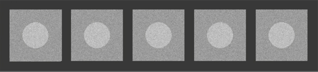
Test images are synthetically generated (Zhang, 1993b). They are of size 256 × 256 with 256 gray levels. The objects are centered discs of various sizes with gray-level 144. The background is homogeneous with gray-level 112. These images are then added by independent zero-mean Gaussian noise with various standard deviations. To cope with the random nature of the noise, for each standard deviation five noise samples are generated independently and are added separately to the noise-free images in this study. Five generated test images form a test group. Figure 2.21 gives an example.
Test images are segmented by thresholding them as described earlier. A sequence of 14 threshold values is taken to segment each group of images. The five evaluation methods are then applied to the segmented images. The values of their corresponding measurements are obtained by averaging the results of the five measurements over each group. In Figure 2.22, the curves corresponding to different measurement values are plotted.
Discussions
These curves can be analyzed by comparing their forms. First, as the worst segmentation results provide the highest value for all measurements, the valley values that correspond to the best segmentation results determine the margin between the two extremes. The deeper the valley, the larger the dynamic range of measurements for assessing the best and worst segmentation results. Comparing the depth of valleys, these methods can be ranked in the order of D-AA, D-PE, D-ND, G-GU, and G-GC. Note that the G-GC curve is almost unity for all segmented images, which indicates that different segmentation results can hardly be distinguished in such a case.
Secondly, for the evaluation purpose, a good method should be capable of detecting very small variations in segmented images. The sharper the curves, the higher the measure’s discrimination capability to distinguish small segmentation degradation. The ranking of these five methods according to this point is the same as above. If looking at more closely, it can be seen that although D-AA and D-PE curves are parallel or even overlapped for most of the cases in Figure 2.22, the form of the D-AA curve is much sharper than that of the D-PE curve near the valley. This means that D-AA has more power than D-PE to distinguish those slightly different from the nearly best segmentation results, which is more interesting in practice. It is clear that D-AA should not be confused with D-PE. On the other hand, the flatness of the G-GC and G-GU curves around the valley show that the methods based on the goodness measurements such as GC and GU are less appropriate in segmentation evaluation.
The effectiveness of evaluation methods is largely determined by their employed image quality measurements (Zhang, 1997c). From this comparative study, it becomes evident that the evaluation methods using discrepancy measurements such as those based on the feature values of segmented objects and those based on the number of misclassified pixels are more powerful than the evaluation methods using other measurements. Moreover, as the methods compared in this study are representative of various method subgroups, it seems that the empirical discrepancy methods surpass the empirical goodness methods in evaluation.

2.5Problems and Questions
![]()
2-1Search in the literature, find some new image segmentation algorithms, classify them into four groups according to Table 2.1.
2-2Show that the Sobel masks can be implemented by one pass of the image by using mask [–101] and another pass of the image by using mask [12 1]T.
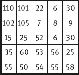
2-3Given an image as shown in Figure Problem 2-3, compute gradient maps by using Sobel, Isotropic, and Prewitt operators, respectively. What observations can you make from the results?
2-4*What is the cost value of the minimum-cost path in Figure 2.7?
2-5An image is composed of an object whose gray-level mean is 200 and the variance is 200 on a background whose gray-level mean is 20 and the variance is 20. What is the optimal threshold value for segmenting this image? Could you propose another technique to solve this problem?
2-6The coordinates of the three vertices of a triangle are (10, 0), (10,10), (0,10), respectively. Give the Hough transforms for the three edges of this triangle.
2-7Extend the Hough transform technique to detect 2-D lines to the Hough transform technique to detect the 3-D plane.
2-8Compute the subpixel location, using separately the moment-preserving method and the expectation of first-order derivatives method, for the input sequence, which is 0.1, 0.1, 0.1, 0.15, 0.25, 0.65, 0.75, 0.85, 0.9, 0.9.
2-9For the shape shown in Figure Problem 2-9, construct its R-table.

2-10*Suppose that an image is segmented by two algorithms, A and B, respectively. The results are shown in Figure Problem 2-10, respectively (bold letters belong to the objects). Use two criteria (the goodness based on intra-region uniformity and the goodness based on inter-region contrast) to judge the two-segmentation results and compare the performances of A and B.
2-11Generate an image with an irregular object in it. Add some zero-mean Gaussian noise to this image. Select the standard deviation of the Gaussian noise as the gray-level difference between the average value of the object and the average value of the background. Segment this image with any thresholding technique, and judge the segmentation result using the probability of the error.
2-12Repeat Problem 2-11 with the absolute UMA and relative UMA defined in eqs. (2.42) and (2.43), respectively.
2.6Further Reading
![]()
1.Definition and Classification
–Image segmentation is a basic type of image technique. Chapters on segmentation can be found in most image processing and computer vision textbooks; for example, Ballard (1982), Castleman (1996), Jähne (1997), Forsyth (2003), and Sonka (2008).
–Research on image segmentation has attracted a lot of attention for more than 50 years (Zhang, 2006d; 2008d; and 2015d). A large number of papers (several thousands) on segmentation research can be found in the literature. Many surveys and reviews have been published, see Zhang (2006b) for a list.
–Related research is far from maturation. To our knowledge, only very few books/monographs specialize in image segmentation: Medioni (2000), Zhang (2001c, 2006b).
–Some segmentation techniques have been designed for special purposes. For example, CBIR or CBVIR (Zhang, 2005c; 2008e).
2.Basic Technique Groups
–Edge detection is the first step in detecting the edges between different parts of an image, and thus decomposing an image into its constitutional components in 1965 (Roberts, 1965).
–The joint effect of the edge orientation and offset over the full range of significant offsets is studied to investigate fully the behavior of various differential edge operators, such as Sobel, Prewitt, and Robert’s cross operators (Kitchen, 1989).
–An analytical study of the effect of noise on the performance of different edge operators can be found in the study of He (1993).
–Thresholding is the most frequently used segmentation technique. Some survey and evaluation papers are Weszka (1978), Sahoo (1988), Zhang (1990), and Marcello (2004).
–An example of color image segmentation can be found in Dai (2003,2006).
–A comparison of several typical thresholding techniques in Xue (2012).
3.Extension and Generation
–An analytical study of the magnitude and direction response of various 3-D differential edge operators can be found in Zhang (1993c).
–The determination of the subpixel edge location is an approximation/estimation process based on statistical properties. Some error analysis for the technique using tangent direction information can be found in Zhang (2001c).
–Other than the techniques discussed in this chapter, there are other techniques for the subpixel edge location. For example, a technique using a small mask to compute orthogonal projection has been presented in Jensen (1995).
–An extension from object to object class in segmentation can see Xue (2011).
4.Segmentation Evaluation
–Segmentation evaluation has obtained many attention in recent years, and general review of the related progress can be found in Zhang (2006c, 2008c, and 2015c).
–An evaluation and comparison experiment for different types of segmentation algorithms can be found in Zhang (1997b).
–In Section 2.4, the presentation and description of evaluation uses still images as examples. Many approaches discussed there can also be applied to the evaluation of video. There are also techniques specialized for video; for example, see Correia (2003).
–The systematic study of segmentation evaluation is one level up from segmentation evaluation itself. Little effort has been spent on it. The first general overview is Zhang (1996c). Some more references can be found in Zhang (1993a, 2001c, 2008c, and 2015c).
–The purpose of segmentation evaluation is to guide the segmentation process and to improve the performance in the segmenting images. One approach using the evaluation results to select the best algorithms for segmentation with the framework of expert system is shown in Luo (1999) and Zhang (2000c).