
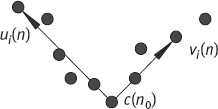
1.Defining alternative curvature measurements based on the angles between vectors This approach consists of estimating the angle defined at c(n0) by vectors along the contour. Various estimations differ in the way that these vectors are fitted or by the method that the estimation is applied. Let c(n) = [x(n),y(n)] be a discrete curve. The following vectors can be defined:
These vectors are defined between c(n0) (the current point) and the ith neighbors of c(n) to the left and to the right, as shown in Figure 6.16, where the left and the right vectors represent ui(n) and vi(n), respectively (Costa 2001).
The high curvature points can be obtained by the following equation
where ri(n) is the cosine of the angle between the two vectors ui(n) and vi(n). Therefore, –1 ≤ ri(n) ≤ 1, with ri(n) = –1 for straight lines and ri(n) = 1 when the angle becomes 0° (the smallest possible angle). In this sense, ri(n) can be used as a measurement that is capable of locating high curvature points.
2.Interpolating x(t) and y(t) followed by differentiation
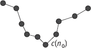
Suppose the curvature at c(n0) is to be estimated. The interpolation approach consists of interpolating the neighbor points around c(n0), as shown in Figure 6.17.
There are different approaches for approximating or interpolating the contour in order to analytically derive the curvature. The simplest approach is to approximate the derivatives of x(n) and of y(n) in terms of finite differences, that is, The curvature can then be estimated by taking the above-calculated values into eq. (6.25). Although this simple approach can be efficiently implemented, it is sensitive to noise.
A more elaborate technique has been proposed (Medioni, 1987), which is based on approximating the contour in a piecewise fashion in terms of cubic B-splines. Suppose that it is required to approximate a contour segment by a cubic parametric polynomial in t, with t € [0,1]. The curve approximating the contour between two consecutive contour points A(t = 0) and B(t = 1) is defined as
where a, b, c, and d are taken as the parameters of the approximating polynomial. By taking the respective derivatives of the above parametric curve into eq. (6.25):
Here, it is supposed that the curvature is to be estimated around the point A(0) (i. e., for A(t = 0)).
6.4.2.4Descriptors Based on Curvatures
While the curvature itself can be used as a feature vector, this approach presents some serious drawbacks including the fact that the curvature signal can be too long (involving thousands of points, depending on the contour) and highly redundant. Once the curvature has been estimated, the following shape measurements can be calculated in order to circumvent these problems.
Curvature Statistics
The histogram of curvatures can provide a series of useful global measurements, such as the curvature’s mean, median, variance, standard deviation, entropy, moments, etc.
Maxima, Minima, and Inflection Points
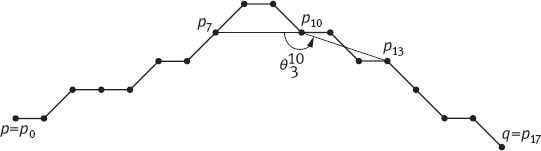
The fact that not all points along a contour are equally important (in the sense of conveying information about the shape) motivates the analysis of dominant points such as those points where the curvature is either a positive maximum, or a negative minimum, or an inflection point. The number of such points, their position along the contour, and their curvature values (in case of maxima and minima curvature points) can be used for shape measurements.
Symmetry Measurement Metric
A symmetry measurement metric for polygonal segments (i. e., curve segments) is defined as
where t is the parameter along the curve, the inner integration is a measurement metric of the angular change until t, A is the total angular change of the curve segment, I is the length of the curve segment, and k(l) can be taken as the curvature along the contour.
Bending Energy
In the continuous case, the mean bending energy, also known as the boundary energy, is defined as
where P is the contour perimeter. The above equation means that the bending energy is obtained by integrating the squared curvature values along the contour and dividing the result by the curve perimeter. Note that the bending energy is also one of the most important global measurements related to the shape complexity.
6.4.2.5 Curvatures on Surfaces
From differential geometry, it is known that the curvature K at a point p on a curve is given by
Curvatures on surfaces are more difficult to define than on planes, as there are infinitely many curves through a point on the surface (Lohmann, 1998). Therefore, it cannot directly generalize the definition of the curvature for planar curves to the curvature of points on a surface. However, it can identify at least one direction in which the curvature is the maximal curvature and another direction in which the curvature is a minimal curvature. Figure 6.18 illustrates this point. These two directions are generally called the principal directions and are denoted t1 and t2. Given the principal directions, it can identify a curve through point p along those directions and employ eq. (6.33) to compute the curvature along these curves. The magnitudes of the curvature along the t1 and t2 directions are denoted k1 and k2.
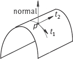
Note that sometimes – for instance, for entirely flat surfaces – more than two principal directions exist. In this case, any arbitrary curve of the maximal or minimal curvature can be used to compute t1 and t2, k1 and k2.
The two principal directions give rise to the following definitions of the curvature on a surface. The term
is called the Gaussian curvature, which is positive if the surface is locally elliptic and negative if the surface is locally hyperbolic. The term
is called the mean curvature. It determines whether the surface is locally convex or concave.
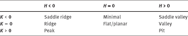
By a combined analysis of the signs of Gaussian curvature K and mean curvature H, different classes of surfaces can be distinguished, as shown in Table 6.3 (Besl, 1988).
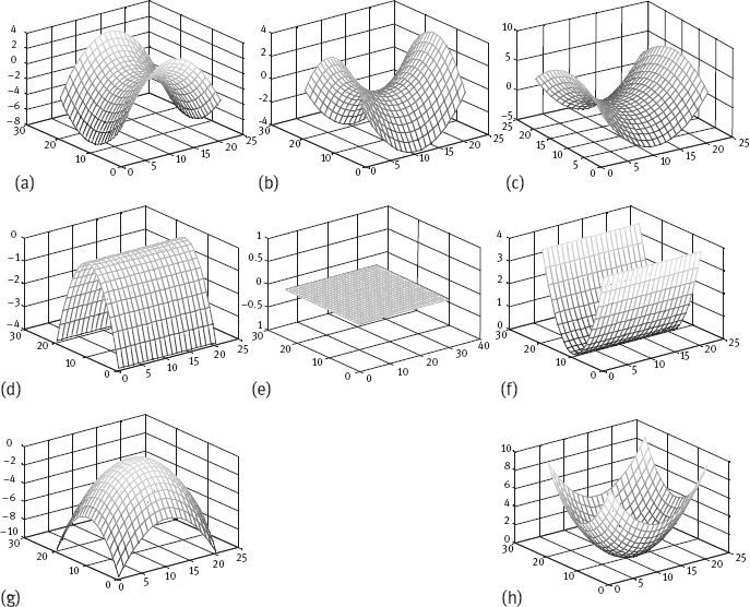
Example 6.2 Eight types of surfaces.
One respect example for each of the eight types of surfaces listed in Table 6.3 are shown in Figure 6.19. The relative arrangement of these examples is same with respect to the relative arrangement in Table 6.3. Figure 6.19(a) is for saddle ridge. Figure 6.19(b) is for minimal. Figure 6.19(c) is for saddle valley. Figure 6.19(d) is for ridge. Figure 6.19(e) is for flat/planar. Figure 6.19(f) is for valley. Figure 6.19(g) is for peak. Figure 6.19(h) is for pit.![]()
Table 6.3: Classification of surfaces according to the signs of curvatures.
6.5Wavelet Boundary Descriptors
Wavelet boundary descriptors are descriptors formed by the coefficients of the wavelet transform of the object boundary.
6.5.1Definition and Normalization
A wavelet family can be defined as
For a given boundary function f(t), its wavelet transform coefficients are
The formula for the reconstruction of f(t) from its wavelet transform coefficients can be written as
where m0 depends on the precision required when the coefficient series is truncated. Suppose the scale function Sm,n(t) is given by Sm,n(t) = 2–m/2Sm,n(2mt–n), and the first term on the right side of eq. (6.38) is represented by a linear combination. Equation (6.38) can be written as
According to the properties of the wavelet transform, the first term on the right side of eq. (6.39) can be considered a coarse map and the second term on the right side of eq. (6.39) corresponds to other details. Name <f, Sm,n> as a scale coefficient and <f, Wm,n> as a wavelet coefficient, both of them together form the wavelet boundary descriptors corresponding to the boundary f(t).
In practical computation of the wavelet boundary transformation, the following points should be considered.
6.5.1.1Normalization for Translation
Scale coefficients and wavelet coefficients have the following relations
Suppose the boundary is translated by δ. The translated boundary is ft (t) = f(t) + δ and
It can be seen from eq. (6.42) that the translation of a boundary has no effect on the wavelet coefficients that describe the details. However, it can be seen from eq. (6.43) that the translation of a boundary has effect on the scale coefficients. In other words, though wavelet coefficients are invariant to translation, translation normalization for scale coefficients is required.
6.5.1.2Normalization for Scale
Suppose the boundary is under scaling by a parameter A. The scaled boundary is fs(t) = Af(t), where the scaling center is also the boundary center. Both scale coefficients and wavelet coefficients are influenced by scaling as
So, a scale normalization with a parameter A for both scale coefficients and wavelet coefficients are required to ensure that the descriptor is invariant to scale change.
6.5.1.3Truncation of Coefficients
If taking all coefficients as descriptors, no boundary information will be lost. However, this may be not needed in practical situations. It is possible to keep all scale coefficients and to truncate certain wavelet coefficients. In such a case, the precision for describing the boundary could be kept at a certain level, which is determined by m0. A high value of m0 causes more details to be lost, while a low value of m0 yields less compression.
6.5.2Properties of the Wavelet Boundary Descriptor
The wavelet boundary descriptor has two basic properties.
1.Uniqueness
The wavelet transform is a one-to-one mapping, so a given boundary corresponds to a unique wavelet boundary descriptor. On the other hand, a wavelet boundary descriptor corresponds to a unique boundary.
2.Similarity measurable
The similarity between two descriptors can be measured by the value of the inner product of the two vectors corresponding to the two descriptors.
Some experiments in the content-based image retrieval framework have been conducted to test the descriptive ability of the wavelet boundary descriptor with the distance between two descriptors.
1.Difference between two boundaries
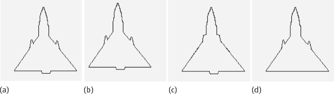
This can be seen in Figure 6.20, in which Figure 6.20(a) is the querying boundary, and Figure 6.20(b-d) is the first three returned results. Distance between two descriptors is computed by first calculating the ratio of the value of the inner product of the two vectors corresponding to the two descriptors and then normalizing the ratio with the maximal possible value of the inner product. The obtained measurement is a percentage of the distance measurement (DIS). The DISs for Figure 6.20(b-d) are 4.25%, 4.31%, and 5.44%, respectively. As the images in Figure 6.20(b, c) are mainly different from Figure 6.20(a) by the position of the boundary, while Figure 6.20(d) is quite different from Figure 6.20(a) by the boundary form, it is evident that the distance between two descriptors is related to the difference between two boundaries.
2.Invariance to the displacement of the boundary
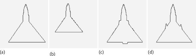
After norm1alization for translation, the wavelet boundary descriptor is invariant to the displacement of the boundary. This can be seen from Figure 6.21, in which Figure 6.21(a) is the querying boundary, and Figure 6.21(b-d) is the first three returned results. The DISs for Figure 6.21(b-d) are 0%, 1.56%, and 1.69%, respectively. From Figure 6.21(b), it can be seen that pure translation has no influence on the distance measurement. From Figure 6.21(c, d), it is evident that some small changes in the form of the boundary have more influence than that caused by translation.
3.Invariance to the scaling of boundary
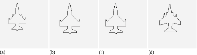
After normalization for the scaling, the wavelet boundary descriptor is invariant to the scaling of the boundary. This can be seen from Figure 6.22, in which Figure 6.22(a) is the querying boundary, and Figure 6.22(b-d) is the first three returned results. The DISs for Figure 6.22(b-d) are 1.94%, 2.32%, and 2.75%, respectively. From Figure 6.22(b), it can be seen that the scale change has little effect on the distance measurement. Compared with Figure 6.22(c) and 6.22(d), the changes in the form of the boundary have more influence than that caused by scale changes.
6.5.3Comparisons with Fourier Descriptors
Compared to Fourier boundary descriptors, wavelet boundary descriptors have several advantages, which are detailed below.
6.5.3.1Less Affected by Local Deformation of the Boundary
A wavelet boundary descriptor is composed of a sequence of coefficients and each coefficient is more locally related to certain parts of the boundary than the coefficients of the Fourier boundary descriptor. The local deformation merely has influence on the corresponding coefficients but no other coefficients.
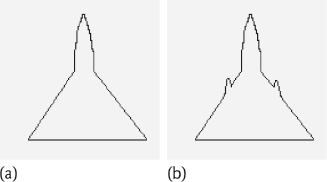
The following experiment is conducted to show this advantage. Two test boundaries are made with a tiny difference in two locations, as shown in Figure 6.23(a, b).
Suppose the descriptor for boundary A is {xa} and {ya}, the descriptor for boundary B is {xb} and {yb}, and their difference is defined as δ2 = (xa – b)2 + (ya – yb)2. Figures 6.24 and 6.25 show this difference for the wavelet boundary descriptor and the Fourier boundary descriptor, respectively. In both figures, the horizontal axis corresponds to the number of coefficients (started from the top of boundary), and the vertical axis is for the difference.


It is easy to see that the local deformation of the boundary causes a quite regular and local change of the difference in the wavelet coefficients as shown in Figure 6.24, while this deformation of the boundary causes a quite irregular and global change of the difference in the Fourier coefficients as shown in Figure 6.25.
6.5.3.2More Precisely Describe the Boundary with Fewer Coefficients
One example is given in Figure 6.26, where Figure 6.26(a) shows an original boundary and the reconstructed boundary with 64 wavelet coefficients and Figure 6.26(b) shows the same original boundary and the reconstructed boundary with 64 Fourier coefficients. The Fourier coefficients just provide the information on 64 discrete points. To get more information that is precise on the boundary, more coefficients are needed.
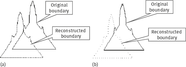

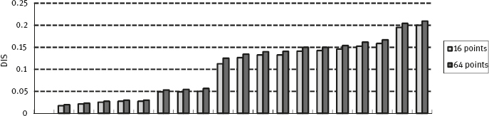
Figure 6.27 shows the results of using only 16 wavelet coefficients for representing the original boundary and for reconstructing the boundary. With fewer coefficients, the descriptive precision is decreased (e. g., sharp angle becomes rounded), but the retrieval performance is less influenced.
Figure 6.28 gives the values of DIS for the first 20 returned results with 64 coefficients and 16 coefficients, respectively. It can be seen that the change in the DIS values with fewer coefficients is not very significant.
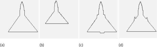
Figure 6.29 provides the retrieval results using 16 coefficients of a wavelet boundary descriptor. Figure 6.29(a) is the querying boundary, and Figure 6.29(b-d) is the first three returned results. The DISs for Figure 6.29(b-d) are 1.75%, 2.13%, and 2.50%, respectively. Though the DIS values here have some difference with respect to Figure 6.22, the retrieved boundary images are exactly the same. It seems that, with fewer coefficients, the boundary can still be described sufficiently.
6.6Fractal Geometry
Fractal geometry is a tool to study irregularities. It can also describe self-similarity. As far as shape analysis is concerned, fractal measurements are useful in problems that require complexity analysis of self-similar structures across different scales (Costa, 2001).
6.6.1Set and Dimension
There are two possible distinct definitions of the dimension of a set in the Euclidean space RN.
1.The topological dimension coincides with the number of degrees of freedom that characterize a point position in the set, denoted dT. Therefore, the topological dimension is 0 for a point, 1 for a curve, 2 for a plane, and so on.
2.The Hausdorff-Besicovitch dimension,d, was formulated in 1919 by the German mathematician Felix Hausdorff.
For a set in RN, it has d ≥ dT. Both of the two dimensions are within the interval [0, N]. The topological dimension always takes an integer value, which is not necessarily the case for the Hausdorff–Besicovitch dimension. In the case of planar curves (such as image contours), the Hausdorff–Besicovitch dimension is an important concept that can be applied to complexity analysis, where the closer d is to 2, the more the curve fills the plane to which it belongs. Therefore, this dimension can be used as a curve complexity measurement.
The notion of a fractal set is defined as a set whose Hausdorff-Besicovitch dimension is greater than its topological dimension Mandelbrot (1982). Since d can take a non-integer value, the name fractal dimension is used. It is nevertheless important to say that the formal definition of the Hausdorff-Besicovitch dimension is difficult to introduce and hard to calculate in practice. Therefore, alternative definitions for the fractal dimension are taken into account. Frequently, these alternative definitions lead to practical methods to estimate the fractal dimensions of experimental data.
6.6.2The Box-Counting Approach
Let S be a set in R2, and M(r) be the number of open balls of a radius r that are necessary to cover S. An open ball of a radius r centered at (x0, y0), in R2, can be defined as a set of points {(x,y) ϵ R2|[(x – x0)2 + (y – y0)2]1/2 < r}. The box-counting fractal dimensiond is defined as
Therefore, the box-counting dimension is defined in terms of how the number of open balls, which are necessary to cover S, varies as a function of the size of the balls (the radius r, which defines the scale).
An example of how the box-counting dimension can be used in order to define the fractal dimension of Koch’s triadic curve is illustrated in Figure 6.30. As shown in the figure, this curve can be constructed from a line segment by dividing it into three identical portions and substituting the middle portion by two line segments having the same length. The complete fractal curve is obtained by recursively applying ad infinitum the above construction process to each of the four resulting segments. Figure 6.30 shows the results of the four sequential steps of the Koch curve construction process. The self-similarity property of fractal structures stems from the fact that these structures are similar irrespective of the spatial scale used for their visualization.
Recall that the definition of the box-counting dimension involves covering the set with M(r) balls for each radius r. While analyzing the Koch curve, 1-D balls that cover the line segments are taken. For the sake of simplicity, a unit length is also assumed for the initial line segment. Consequently, a single ball of the radius r = 1/2 is needed to cover the Koch curve segment (see Figure 6.31(a)). In the case where smaller balls are used, when r = 1/6, M(r) = 4 balls are needed to cover the Koch curve; whereas, when r = 1/18, a total number of M(r) = 16 balls is required, as illustrated in Figure 6.31(b, c). An interesting conceptual interpretation of this effect is as follows. Suppose the line segments of Figure 6.31(a–c) represent measuring devices with the smallest measuring units. This means that, if one chooses to measure the Koch curve in Figure 6.31 with the measuring device of a length 1, the conclusion is that the length of the curve is 1.
This is because that it cannot take into account the details that are less than 1. On the other hand, if a measuring device with a length 1/3 were used instead, four segments would be needed, yielding a total length of 4(1/3) ≈ 1.33. Table 6.4 summarizes this measuring process of M(r) as a function of r.


Table 6.4: The number M(r) for balls of radius r necessary to cover the Koch curve in Figure 6.30.
| r | M(r) | Measured curve length |
| 1/2 = (1/2)(1) = (1/2)(1/3)° | 1= 4 0 | 1 |
| 1/6 = (1/2)(1/3) = (1/2)(1/3)1 | 4 = 41 | 1.33 |
| 1/18 = (1/2)(1/9) = (1/2)(1/3)2 | 16 = 42 | 1.78 |
| ……… | ……… |
This analysis indicates that when r is decreased by a factor of 1/3, M(r) is increased by a factor of 4. From eq. (6.46), this means that
Therefore, it has d = log(4)/ log(3) ≈ 1.26, which actually is the fractal dimension of the Koch curve. The Koch curve is exactly self-similar, as it can be constructed recursively by applying the generating rule, which substitutes each segment by the basic element in Figure 6.27(b), as explained above.
6.6.3Implementing the Box-Counting Method
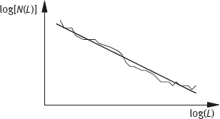
The basic algorithm for estimating the box-counting dimension is based on partitioning the image into square boxes of size L × L and counting the number N(L) of boxes containing at least a portion (whatever small) of the shape. By varying L (the sequence of the box sizes, starting from the whole image, is usually reduced by 1/2 from one level to the next), it is possible to create the plot representing log[N(L)] versus log(L). The fractal dimension can then be calculated as the absolute value of the slope of the line interpolated to the log[N(L)] versus log(L) plot, as illustrated in Figure 6.32. The sequence of the box sizes, starting from the whole image, is usually reduced by 1/2 from one level to the next.
It is important to note that truly fractal structures are idealizations that neither exist in nature nor can be completely represented by computers. The main reasons for this are (1) ad infinitum self-similarity is never verified for shapes in nature (both at the microscopic scale, where the atomic dimension is always eventually achieved, and the macroscopic scale, since the shape has a finite size) and (2) the limited resolution adopted in digital imaging tends to filter the smallest shape detail. Therefore, it is necessary to assume that “fractal” shapes present limited fractality (i. e., they are fractal with respect to a limited scale interval).
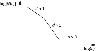
This is reflected in the log[N(L)] versus log(L) plot in Figure 6.33 by the presence of three distinct regions (i. e., a non-fractal region (d ≈ 1),a fractal region (d > 1), and a region with the dimension of zero (d ≈ 0)). This general organization of the curve can be easily understood by taking into account the relative sizes of the boxes and the shape. When the boxes are too small, they tend to “see” the shape portions as straight lines, yielding a dimension of 1. As the size of the boxes increases, the complex details of the shape start to become perceived, yielding a fractal dimension, which is possibly greater than 1 and less than or equal to 2. Finally, when the boxes become too large, the whole shape can be contained within a single box, implying a dimension of zero. Consequently, the line should be fitted to the fractal portion of the log(N(L)) versus log(L) plot in order to obtain a more accurate estimation of the limited fractal behavior of the shape under analysis.
6.6.4Discussions
The fractal dimension attempts to condense all of the details of the boundary shape into a single number that describes the roughness in one particular way. There can be an unlimited number of visually different boundary shapes with the same fractal dimension or local roughness(Russ, 2002).
The fractal dimension of a surface is a real number greater than 2 (the topological dimension of the surface) and less than 3 (the topological dimension of the space in which the surface exists). A perfectly smooth surface (dimension 2.0) corresponds to the Euclidean geometry, and a plot of the actual area of the measured area as a function of the measurement resolution would not change. However, for real surfaces, an increase in the magnification or a decrease in the resolution with which it is examined will reveal more nooks and crannies and the surface area will increase. For a surprising variety of natural and man-made surfaces, a plot of the area as a function of the resolution is linear on a log-log graph, and the slope of this curve gives the dimension d. As the measurement resolution becomes smaller, the total measured area increases.
6.7Problems and Questions
![]()
6-1In Section 6.1, several definitions for a shape were given. What are their common points? What are their differences? Provide some examples to show the application areas for each of them.
6-2Given a square and a circle with the same area. Can they be distinguished by using the form factor, sphericity, circularity, and eccentricity?
6-3*In Figure Problem 6-3, a circle is approximated by an octant formed by discrete points. Compute the form factor, sphericity, circularity, and eccentricity of the octant.

6-4What are the meanings of points, lines, and circles in Figure 6.7?
6-5Prove the following two conclusions for a digital image.
(1)If the boundary is 4-connected, and then the form factor takes the minimum value for an octant region.
(2)If the boundary is 8-connected, and then, the form factor takes the minimum value for a diamond region.
6-6If the boundary of a region in a digital image is 16-connected, what region form gives the minimum value for the form factor?
6-7Provide some examples to show that the six simple descriptors listed in Section 6.3 reflect the complexity of the region form.
6-8Compute the shape number for three regions in Figure 6.4 and compare them. Which two are more alike?
6-9Following the examples in Figure 6.11, draw the horizontal projection and vertical projection of 26 capital English letters that are represented by 7 × 5 dot-matrix:
(1)Compare the horizontal projection and vertical projection. What are their particularities?
(2)Using only these projections, can the 26 capital English letters be distinguished?
6-10Back to the octant in Figure Problem 6-3:
(1)Compute its curvatures (take k = 1,2,3);
(2)Compute the corresponding bending energy.
6-11Can the fractal dimension be used to distinguish a square from a circle?
6-12*Consider the pattern sequence in Figure Problem 6-12. The left pattern is a square, and dividing it into nine equal small squares and removing the central small square yields the middle pattern in Figure Problem 6-12. Further dividing the rest of the eight squares into nine equal small squares and removing the central small square yields the right pattern in Figure Problem 6-12. Continuing this way, a square with many holes (from big ones to small ones) can be obtained. What is the fractal dimension of this square?

6.8Further Reading
![]()
1.Definitions and Tasks
–One deep study on shape analysis based on contours can be found in Otterloo (1991).
–An application of the wavelet-based shape description for image retrieval can be found in Yao (1999).
2.Different Classes of 2-D Shape
–Shape classification is still studied widely, and some discussions can be found in Zhang (2003b).
3.Shape Property Description
–Detailed discussion on the form factor of an octagon can be found in Rosenfeld (1974).
–The computation of data listed in Table 6.1 can be found in Zhang (2002b).
4.Technique-Based Descriptors
–The computation of curvature for 3-D images can be found in Lohmann (1998).
–The structure information of a region has close relation with the shape information and the relationship among objects (Zhang, 2003b).
5.Wavelet Boundary Descriptors
–More details on the wavelet boundary descriptors can be found in Zhang (2003b).
6.Fractal Geometry
–Besides box-counting methods, another method for computing fractal dimensions is based on the area of influence or the area of spatial coverage (Costa, 1999; 2001).
–According to fractal dimensions, 2-D signatures can be described (Taylor, 1994).