
where k + 1 is mod K. The first term corresponds to the vertical and horizontal components, while the second term corresponds to the diagonal components.
3.5.1.2Boundary Diameter
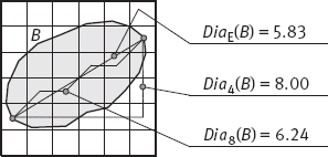
The diameter of a boundary B is defined as
where D is a distance measurement. The value of the diameter and the orientation of a line segment connecting the two extreme points that comprise the diameter (this line is called the major axis of the boundary) are useful descriptors of a boundary. The minor axis of a boundary is defined as the line perpendicular to the major axis, of such a length that a box passing through the outer four points, where the boundary is intersected with the two axes, completely encloses the boundary. This box is called the basic rectangle, and the ratio of the major to the minor axis is called the eccentricity of the boundary, which is also a useful descriptor.
One example of the diameter of a boundary is shown in Figure 3.25. Note that the diameter can be measured using different distance metrics (such as Euclidean, city-block, chessboard, etc.) and with different results.
3.5.1.3Boundary Curvature
The curvature of a curve is defined as the rate of the change of the slope. As the boundary is traversed in the clockwise direction, a vertex point p is said to be part of a convex segment if the change in the slope at p is nonnegative; otherwise, p is said to belong to a segment that is concave. In general, obtaining a reliable measurement of curvature at a point in a digital boundary is difficult because these boundaries tend to be locally “ragged.” However, using the difference between the slopes of adjacent boundary segments (which have been represented as straight lines) as a descriptor of the curvature at the point, where the segments intersect, sometimes has proven to be useful.
For 3-D images, surface curvature is defined by two maximum and minimum radii. If both are positive as viewed from “inside” the object bounded by the surface, the surface is convex. If both are negative, the surface is concave, and if they have opposite signs, the surface has a saddle curvature. Figure 3.26 shows one example for each case, where Figure 3.26(a) is for convex, Figure 3.26(b) is for concave, and Figure 3.26(c) is for saddle. The total integrated curvature for any closed surface around a simply connected object (no hole, bridge, etc., exist) is always 4π.
3.5.2Shape Numbers
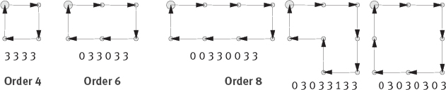
Shape number is a descriptor for the boundary shape based on chain codes. According to the starting point, a chain-coded boundary has several first-order differences, in which one with the smallest value is the shape number of this boundary. For example, in Figure 3.4, the chain code for the boundary before normalization is 10103322, the difference code is 3133030, and the shape number is 03033133.
The order n of a shape number is defined as the number of digits in its representation. For a closed boundary, n is even. The value of n limits the number of different shapes of a boundary that are possible. Figure 3.27 shows all the shapes of orders 4, 6, and 8.

In practice, for a desired shape order, the shape number of a boundary can be obtained as follows:
1.Select the rectangle whose long/short axis ratio is the closest to the given boundary, as shown in Figure 3.28(a, b).
2.Divide the selected rectangle into multiple squares (grids) according to the given order, as shown in Figure 3.28(c).
3.Select the squares such that each square has more than 50% of its area inside the boundary and a polygon that fits best to the boundary is built by these squares, as shown in Figure 3.28(d).
4.Start from the black point in Fig. 3.28(d) and obtain its chain codes, as shown in Figure 3.28(e).
5.Obtain the first-order differences of the chain codes, as shown in Figure 3.28(f).
6.Obtain the shape number of the boundary from its first-order differences, as shown in Figure 3.28(g).
3.5.3Boundary Moments
The boundary of an object is composed of a number of segments. Each segment can be represented by a 1-D function f(r), where r is an arbitrary variable. Further, the area under f(r) can be normalized and counted as a histogram. For example, the segments in Figure 3.29(a) with L points can be represented as a 1-D function f(r), as shown in Figure 3.29(b).

The mean of f(r) is given by
The nth boundary moment of f(r) about its mean is
Here, μn is directly related to the shape of f(r). For example, μ2 measures the spread of segments about its mean and μ3 measures the symmetry of segments with respect to its mean. These moments are not depend on the position of segments in space, and are not sensitive to the rotation of the boundary.
3.6Descriptors for Regions
The common properties of a region include geometric properties such as the area of the region, the centroid, and the extreme points; shape properties such as measurements of the circularity and elongation; topological properties such as the number of components and holes, and intensity properties such as mean gray tone and various texture statistics (Shapiro, 2001). Some of them are briefly discussed in the following.
3.6.1Some Basic Descriptors
Region descriptors describe the properties of an object region in images. Some of them can be computed and obtained easily, such as the area and centroid of an object, as well as the density of an object region.
3.6.1.1Area of Object
The area of an object region provides a rough idea about the size of the region. It can be computed by counting the number of pixels in the region:
Given a polygon Q whose corners are discrete points, let R be the set of discrete points included in Q. Let NB be the number of discrete points that lie exactly on the polygonal line that forms the borders of Q and let NI be the number of interior points (i.e., non-border points) in Q. Then, |R| = NB + NI. The area of Q, denoted A(Q), is the number of unit squares (possibly fractional) that are contained within Q and is given by Marchand (2000)
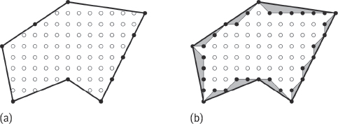
Consider the polygon Q shown in Figure 3.30(a). The border of Q is represented as a continuous bold line. Points in Q are represented by discs (black • and white °). Black discs represent border points (i.e., corners and points that lie exactly on the border of Q). Empty (white) discs represent interior points. Clearly, NI = 71 and NB = 10. Therefore, A(Q) = 75.
It is necessary to distinguish the area defined by a polygon Q and the area defined by the contour of P, which is defined from the border set B. Figure 3.30(b) illustrates the resulting contour obtained when 8-connectivity is considered in P and 4-connectivity is considered in Pc. The area of P is clearly 63. One can verify that the difference between this contour-enclosed set and A(Q) is exactly the area of the surface between the contour and Q (shaded area).
3.6.1.2Centroid of Object
It is often useful to have a rough idea of where an object region is in an image. Centroid indicates the mass center of an object and the coordinates of a centroid are given by

In cases when the scale of objects is relatively small compared to the distance between objects, the object regions can be approximately represented by a point located at the centroid.
For an irregular object, its centroid and geometric center are often different. One example is given in Figure 3.31, where the centroid is represented by a square, the intensity weighted centroid is represented by a star, and the geometric center determined by the circumscribed circle is represented by a round point.
3.6.1.3Region Density
Density (Densitometric) features are different from geometric features in that they must be computed based on both the original (grayscale) images and segmented images. Density is often represented in an image by gray levels. Commonly used region density features include maximum, minimum, mean, and average values as well as variance and other high order moments. They can be obtained from the gray-level histogram.
Several typical density feature descriptors are listed as follows:
1.Transmission (T): It is the proportion of incident light that passes through the object.
2.Optical density (OD): It is defined as the logarithm (base 10) of the ratio of incident light to the transmitted light (that is, the reciprocal of transmission).
OD is related directly to absorption, which is a complementary of transmission. Because absorption is multiplicative rather than additive, a logarithmic scale for absorption is useful to allow values of two or more absorbing items to be added simply. The value of OD goes from 0 (100% transmission) to infinity (zero transmission, for a completely opaque material).
3.Integrated optical density (IOD): It is a commonly used region gray-level feature. It is the summation of the pixel’s OD for the whole image or a region in the image. For an M × N image f(x, y), its IOD is
Denoting the histogram of an image H(•) and the total number of gray-levels G,
IOD is the weighted sum of all gray-level bins in the histogram.
4.Statistics of the above three descriptors, such as median, mean, variance, maximum, and minimum.
3.6.1.4Invariant Moments
For a 2-D discrete region f(x, y), its (p + q)th moment is defined as (Gonzalez 2002)
It has been proven that mpq is uniquely determined by f(x, y). On the other hand, mpq also uniquely determines f(x, y).
The moments around the center of gravity are called central moments. The (p + q)th central moment is defined by
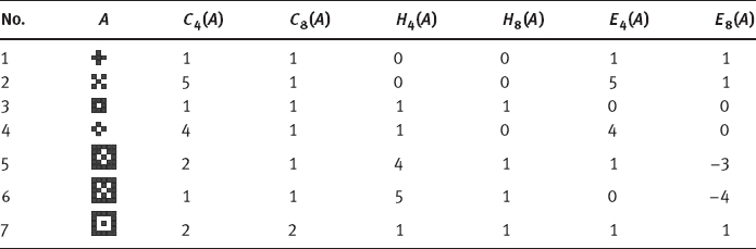
where x = m10/m00 and ȳ = m01/m00 are just the centroid coordinates defined in eqs. (3.22) and (3.23). Sample values of the first five moments for some simple images (the coordinate center is at the center of the image, pixels have unit size) shown in Figure 3.32 are given in Table 3.3 (Tomita, 1990).
The normalized central moment (normalization with respect to object area) of f(x, y) is defined by

Table 3.3: The first five moments for images shown in Figure 3.32.

The following seven moments that are invariants to translation, rotation, and scaling are composed by normalized second and third central moments:
Figure 3.33 gives one example to show the invariance of the above seven invariant moments. In Figure 3.33, Figure 3.33(a) is the original test image, Figure 3.33(b) is that image after 45° rotation counterclockwise, Figure 3.33(c) is that image reduced to half size, and Figure 3.33(d) is the mirror image of Figure 3.33(a). The seven moments defined in eqs. (3.30–3.36) are computed for all four images, and the results are listed in Table 3.4. The four values for each moment are quite close with some small differences that can be allocated to round-off in computation.
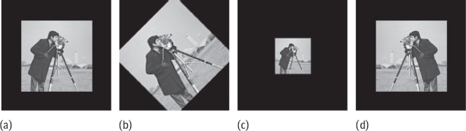
Table 3.4: Some test results of invariant moments.

The above-discussed seven invariant moments are suitable for describing regions. They can also be used to describe the region boundary, but a modification is necessary (Yao, 1999). For a region f(x, y), under a scale change, x′ = kx, y′ = ky, its moments are multiplied by kpkqk2. The factor k2 is related to the area of an object. The center moments of f(x′, y′) become The normalized moments are defined as
In order to make the normalized moments invariant to scaling, let and then
For a boundary, scaling causes the change of the perimeter of the boundary. The change factor is not k2 but k. The center moments now become In order to make the normalized moments invariant to scaling, let and
3.6.2Topological Descriptors
Topology is the study of properties of a figure (object) that are unaffected by any deformation, as long as there is no tearing or joining of the figure (sometimes these are called rubber-sheet distortions). Topological properties do not depend on the notion of distance or any properties implicitly based on the concept of a distance measurement. Topological properties are useful for global descriptions of regions.
3.6.2.1Euler Number and Euler Formula
Two topological properties that are useful for region description are the number of holes in the region and the number of connected components in the region (Gonzalez, 2002). The number of holes H and the number of connected components C in a 2-D region can be used to define the Euler number E:

The Euler number is a topological property. The four letters shown in Figure 3.34 have Euler numbers equal to –1, 2, 1, and 0, respectively.
For an image containing Cn different connected foreground components and assuming that each foreground component Ci contains Hi holes (i. e., defines Hi extra components in the background), the Euler’s number (a more generalized version) associated with the image is calculated as
There are two Euler numbers for a binary image A, which are denoted E4(A) and E8(A) (Ritter, 2001). Each is distinguished by the connectivity used to determine the number of feature pixel components and the connectivity used to determine the number of non-feature pixel holes contained within the feature pixel connected components.
The 4-connected Euler number, E4(A), is defined to be the number of four-connected feature pixel components minus the number of 8-connected holes, which is given by
Here, C4(A) denotes the number of 4-connected feature components of A and H8(A) is the number of 8-connected holes within the feature components.
The 8-connected Euler number, E8(A), is defined by
where C8(A) denotes the number of 8-connected feature components of A and H4(A) is the number of 4-connected holes within the feature components.
Table 3.5 shows Euler numbers for some simple pixel configuration (Ritter, 2001).
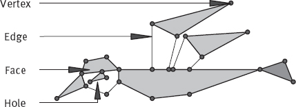
Regions represented by straight-line segments (referred to as polygonal networks) have a particular simple interpretation in terms of the Euler number. Denoting the number of vertices by V, the number of edges by Q, and the number of faces by F, the following relationship can be derived, which is called the Euler formula,
The drawing in Figure 3.35 is an example of polygon network and has 26 vertices, 33 edges, 7 faces, 3 connected regions, and 3 holes. Therefore, its Euler number is 0.
Table 3.5: Examples of pixel configurations and Euler numbers.
3.6.2.2Euler Number in 3-D
Some terms need to be defined first (Lohmann, 1998). A cavity is a completely enclosed component of the background. A handle has sometimes been identified by the concept of a “tunnel,” which is a hole having two exits to the surface. The “number of handles” is also called the “number of tunnels,” “first Betti-Number,” or “genus.”
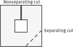
The genus counts the maximum number of non-separating cuts it can make through the object without producing more connected components, where a “cut” must fully penetrate the object. Figure 3.36 shows examples of such cuts. There are many numbers of separating and nonseparating cuts conceivable for this object. But once you have decided on one particular nonseparating cut, no further non-separating cuts are possible since any further cut will slice the object into two. Therefore, the genus for this object is one. An object consisting of two crossed rings has a genus of 2, because there are two nonseparating cuts possible, one for each component.
Now, the 3-D Euler number is defined as the number of connected components (C) plus the number of cavities (A) minus the genus (G):
The Euler number is clearly a global feature of an object. However, it is possible to compute both the Euler number and the genus by purely local computations (i.e., by investigating small neighborhoods).
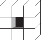
The genus of a digital object can be computed by investigating the surfaces that enclose the object and its cavities. If the object is digital, the enclosing surfaces consist of a fabric of polyhedral. Such surfaces are called netted surfaces. They are made by numbers of vertices (V), edges (Q), and faces (F) of voxels. The genus of a netted surface has the property given by
In Figure 3.37, F = 32, Q = 64, and V = 32. So, 2 – 2G = 32 – 64 + 32 = 0, that is, G = 1.
Sometimes, it may happen that two closed netted surfaces meet at a single edge. Such edges are counted twice – once for each surface they belong to.
Each connected component and cavity is wrapped up in a netted surface Si. If there are M number of connected components and N number of cavities, the number of such surfaces will be M + N. Each of the closed surfaces encloses a single connected component or a single cavity. According to eq. (3.46), since Ei = 1 – Gi,
Let S denote the image foreground, S′ denote its background, and Ek, k = 6, 26 denote the Euler number of a k-connected object, then the following two duality formulas exist