7.5.1.3Mean Shift and Kernel Tracking

Mean shift refers to the mean vector shifting. It is a nonparametric technique that can be used to analyze complex multimodal feature spaces and determine feature clustering. Mean shift technique can also be used to track moving objects; in this case, the region of interest corresponds to the tracking window, while the feature model should be built for tracked object. The basic idea in using mean shift technique for object tracking is to move and search the object model within the tracking window, and to calculate the correlation place with largest value. This is equivalent to determine the cluster center and move the window to the position coincides with the center of gravity (convergence).

To continuously track object from the previous frame to the current frame, the object model determined in the previous frame can be put on the center position xc of local coordinate system in the tracking window, and let the candidate object in current frame be at position y. Description of the property of the candidate object can be characterized by taking advantage of the probability density function p(y) estimated from the data out of current frame. The object model Q and the probability density function of candidate object P(y) are defined as follows:

$\text{Q}=\left\{q_v\right\}{\displaystyle {\sum }_{v=1}^m{q}_v=1}\left(7.52\right)$

$P\left(y\right)=\left\{p_v\left(y\right)\right\}{\displaystyle {\sum }_{v=1}^m{p}_v=1}\left(7.53\right)$

where v = 1,..., m, m is the number of features. Let S(y) be the similarity function between P(y) and Q:

$S\left(y\right)=S\left\{P\left(y\right),\text{Q}\right\}\left(7.54\right)$

For an object-tracking task, the similarity function S(y) is the likelihood that an object to be tracked in the previous frame is at position y in the current frame. Therefore, the local extreme value of S(y) corresponds to the object position in the current frame.

To define the similarity function, the isotropic kernel can be used (Comaniciu 2000), in which the description of feature space is represented with kernel weights, then S(y) is a smooth function of y. If n is the total number of pixels in the tracking window, wherein xi is the ith pixel location, then the probability estimation for the candidate feature vector Qv in candidate object window is

$\text{<mover accent="true"> Q <mo>^</mo> </mover>}{}_v=C_q{\displaystyle {\sum }_i^{n}K\left(x_i-x_c\right)}\delta \left[b\left(x_i\right)-q_v\right]\left(7.55\right)$

where b(xi) is the value of the object characteristic function at pixel xi; the role of δ function is to determine whether the value of xi is the quantization results of feature vector Qv; K(x) is a convex and monotonically decreasing kernel function; Cq is the normalization constant:

$C_q=1/{\displaystyle {\sum }_{i=1}^{n}K\left(x_i-x_c\right)}\left(7.56\right)$

Similarly, the probability estimation of the feature model vectors Pv for candidate object P(y)

${\widehat{P}}_v=C_p{\displaystyle {\sum }_i^{n}K\left(x_i-y\right)}\delta \left[b\left(x_i\right)-p_v\right]\left(7.57\right)$

where Cp is a normalization constant (for a given kernel function, it can be calculated in advance):

$C_p=1/{\displaystyle {\sum }_{i=1}^{n}K\left(x_i-y\right)}\left(7.58\right)$

Bhattacharyya coefficient is commonly used to estimate the degree of similarity between the density of object mask and the density of candidate region. The more similar the distributions between the two densities is, the greater the degree of similarity. The center of the object position is

$y=\frac{{\displaystyle {\sum }_{i=1}^n{x}_i{w}_{i}K\left(y-x_i\right)}}{{\displaystyle {\sum }_{i=1}^n{w}_{i}K\left(y-x_i\right)}}\left(7.59\right)$

where wi is a weighting coefficient. Note that from eq. (7.59), the analytic solution of y cannot be obtained, so an iterative approach is needed. This iterative process corresponds to a process of looking for the maximum value in neighborhood. The characteristics of kernel tracking method are: operating efficiency is high, easy modular, especially for objects with regular movement and low speed. It is possible to successively acquire new center of the object, and achieve the object tracking.

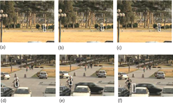
Example 7.6 Feature selection during tracking.

In object tracking, in addition to tracking strategies and methods, the choice of which kinds of object features is also very important (Liu, 2007). One example of using color histogram and edge direction histogram (EOH) under the mean shift framework is shown in Figure 7.15. Figure 7.15(a) is a frame image of a video sequence, in which the object to be tracked has similar color with background, the result obtained with color histogram is unsuccessful as shown in Figure 7.15(b), while the result obtained with edge direction histogram can catch the object as shown in Figure 7.15(c). Figure 7.15(d) is a frame image of another video sequence, in which the edge direction of object to be tracked is not obvious, the result obtained with color histogram can catch object as shown in Figure 7.15(e), while the result obtained with edge direction histogram is not reliable as shown in Figure 7.15(f). It is seen that using a feature alone under certain circumstances can lead to failure of the tracking result.

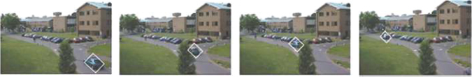
The color histogram mainly reveals information inside object, while the edge direction histogram mostly reflects information of object boundary. Combining the two, it is possible to obtain a more general effect. One example is shown in Figure 7.16, where the goal is to track the moving car. Since there are changes of object size, changes of viewing angle and object partial occlusion, etc., in the video sequence, so the car’s color or outline will change over time. By combining color histogram and edge direction histogram, good result has been obtained.