
8Mathematical Morphology
Mathematical morphology is a form-based mathematical tools suitable for image analysis (Serra, 1982). Its basic idea is to apply some forms of structure elements to measure and to extract the corresponding shape in image, in order to achieve image analysis and identification purposes. The applications of mathematical morphology can simplify image data, maintain their basic shape characteristics, and remove extraneous structures. Mathematical morphology algorithm has also a natural structure for parallel implementation.
The operands of mathematical morphology operation may be a binary image or a gray-scale image. In this chapter, they will be described separately.
The sections of this chapter will be arranged as follows:
Section 8.1 introduces the basic operations of binary image mathematical morphology. First of all, the most fundamental dilation and erosion operations are discussed in detail. On this basis, the opening and closing operations are also discussed. Finally, some basic properties of these basic operations are summarized.
Section 8.2 describes first another basic morphological operation, hit-or-miss transform. Then, some mathematical morphological operations composed of various basic operations for functions such as the construction of region convex hull, the thinning and thickening of region are introduced.
Section 8.3 discusses some practical binary morphological algorithms for specific image applications, such as noise filtering, corner detection, boundary extraction, target location, area filling, connected component extraction, and skeleton computation.
Section 8.4 focuses on the basic operations of mathematical morphology of grayscale image. A generalization from binary analogy is used to bring the basic operations (dilation and erosion, opening and closing) to grayscale image.
Section 8.5 presents some combined morphological operations, including morphological gradients, morphological smoothing, top-hat and bottom-hat transforms, morphological filters and soft morphological filters for grayscale images.
Section 8.6 discusses some practical grayscale morphology algorithms for specific image applications, which can be used for background estimation and removal, morphological detection of edges, fast segmentation of image clustering, watershed segmentation and texture segmentation.
8.1Basic Operations of Binary Morphology
The operands of binary morphology are two sets, generally referred to as image set A and structure element set B (itself is still an image set and simply called structure element), the mathematical morphology operation uses B to operate A. In the following, the shaded region represents region with value 1, and the white region represents region with value 0, the operation is performed on image regions with value 1.
8.1.1Binary Dilation and Erosion
A basic pair of binary morphology operations are dilation and erosion.
8.1.1.1Binary Dilation
The operator of dilation is ⊕, dilating A by B is written A ⊕ B and is defined as
The above equation shows that the process of dilating A by B is first to reflect B around the origin, then to shift this reflection by x, in requiring that the intersection of A and the reflection of B is not an empty set. In other words, the set obtained through dilating A by B is the set of origin positions of B when the displacement of B has at least intersected with a nonzero element in A. According to this explanation, eq. (8.1) can also be written as follows:
This equation can help to understand the concept of dilation by means of a convolution operation. If the B is seen as a convolution mask, dilation is first to reflect B around the origin, then to move continuously its reflection on the image A.
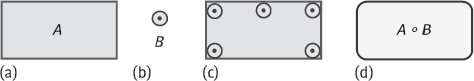
Example 8.1 Illustration of dilation operation.
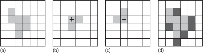
An example of the dilation operation is shown in Figure 8.1. Figure 8.1(a) is the shaded set A, Figure 8.1(b) is the shaded structure element B (the origin is marked with a “+”), the reflection of B is shown in Figure 8.1(c), and in Figure 8.1(d), the two shaded portions (the darker part represents the enlarged part) together form the set A ⊕ B. It is seen that the original region has been expanded by dilation. ![]()
8.1.1.2Binary Erosion
The operator of erosion is ⊖, eroding A by B is written A ⊖ B and is defined as follows:
The above equation shows that the result of eroding A by B is the set of all x, where B after shifting x is still in A. In other words, the result of eroding A by B is a set consists of the origin of B when B is completely included in A. The above equation may also help to understand the erosion operation by means of related concepts.
Example 8.2 Illustration of erosion operation.
A simple example is given in Figure 8.2 for erosion operation, wherein the set A in Figure 8.2(a) and the structure element B in Figure 8.2(b) are the same as in Figure 8.1. The dark shaded region (only) in Figure 8.2(c) provides A ⊖ B, while the light shaded region is the part that was belong to A but now eroded. It is seen that the original region has been shrunk by erosion. ![]()
8.1.1.3Dilation and Erosion with Vector Operations
In addition to the aforementioned intuitive definitions for dilation and erosion, respectively, there are a number of equivalent definitions. These definitions have their own characteristics, such as dilation and erosion operations can be achieved either by vector operation or shift operations, and even more convenient in using a computer to complete dilation and erosion operations in practice.
Look at first the vector operation, considering A and B as vectors, then the dilation and erosion can be expressed as
Example 8.3 Using vector operations to achieve dilation and erosion.
Referring to Figure 8.1, taking the upper left corner of the image as {0, 0}, then A and B can be expressed as: A = {(1, 1), (1, 2), (2, 2), (3, 2), (2, 3), (3, 3), (2, 4)} and B = {(0, 0), (1, 0), (0, 1)}, respectively. Perform dilation using vector operation: A ⊕ B = {(1, 1), (1, 2), (2, 2), (3, 2), (2, 3), (3, 3), (2, 4), (2, 1), (2, 2), (3, 2), (4, 2), (3, 3), (4, 3), (3, 4), (1, 2), (1, 3), (2, 3), (3, 3), (2, 4), (3, 4), (2, 5)} = {(1, 1), (2, 1), (1, 2), (2, 2), (3, 2), (4, 2), (1, 3), (2, 3), (3, 3), (4, 3), (2, 4), (3, 4), (2, 5)}. The result is the same as in Figure 8.1(d). Similarly, if the erosion is obtained with the vector operation: A ⊖ B = {(2, 2), (2, 3)}. Comparing to Figure 8.2(c) can verify the results here. ![]()
8.1.1.4Dilation and Erosion with Shift Operations
Shift operations and vector operations are closely linked, and the sum of vectors is a kind of shift operations. According to eq. (8.2), the shift computing formula for dilation can be obtained via eq. (8.4):
This equation shows that the result of A ⊕ B is the union after shifting A for each b ∈ B. It is also interpreted as dilating A by B is to first shift A by every b and then OR up the results together.
Example 8.4 Dilation by means of shift.
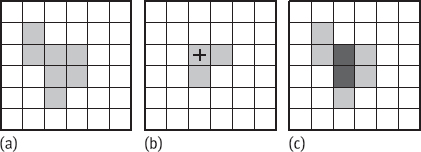
An example of using shift operation to achieve dilation result is shown in Figure 8.3, wherein the set A in Figure 8.3(a) is the same as in Figure 8.1. Figure 8.3(b) is the structure element B. For simplicity, let the pixel at the origin not belong to B, that is, B contains only two pixels. Figure 8.3(c, d) provides the results of shift using the structure element points at the right and below of the origin, respectively. Figure 8.3(e) gives the result obtained by unifying Figure 8.3(c, d), that is, the union of two shaded parts. Comparing it with Figure 8.1(d), except point (1, 1), they are the same. The no-appearance of point (1, 1) in the dilation result is caused by the fact that B does not contain the origin. ![]()
According to eq. (8.2), the shift computing formula for erosion can be obtained via eq. (8.5):

This equation shows that the result of A ⊖ B is the intersection after reversely shifting A for each b ∈ B. It is also interpreted as: eroding A by B is to first reversely shifting A by every b and then AND up the results together.
Example 8.5 Erosion by means of shift.
An example of using shift operation to achieve erosion is shown in Figure 8.4. Wherein Figure 8.4(a, b) is the same as in Fig 8.3. Figure 8.4(c, d) provides the results of reverse shift using the structure element points at the right and below of the origin, respectively. The black region (two pixels) in Figure 8.4(e) gives the result obtained by AND the results in Figure 8.4(c, d). This result is same as that in Figure 8.2(c), so eq. (8.7) is verified. ![]()
The AND set of shifting A by b is also equal to the AND set of shifting B by a, so the eq. (8.6) can be written as:
8.1.1.5Duality of Binary Dilation and Erosion
Dilation and erosion are two operations closely linked, one operation on the image object corresponds to another operation on the image background. According to the relation between the complement (represented by a superscript “c”) and the reflection (represented by the top cap), the duality of dilation and erosion operations can be expressed as:
Example 8.6 Illustration of duality between dilation and erosion.
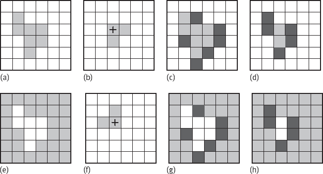
The duality of dilation and erosion can be explained with the help of Figure 8.5. Wherein Figure 8.5(a, b) gives A and B, respectively; Figure 8.5(c, d) gives A ⊕ B and A ⊖ B, respectively; Figure 8.5(e, f) gives Ac and , respectively; Figure 8.5(g, h) gives Ac ⊖ ![]() and Ac ⊕
and Ac ⊕ ![]() (a dark point in the dilation result represents the expanded point, and in the erosion result represents the etched point), respectively. Comparing Figure 8.5(c, g) can verify eq. (8.9), and comparing Figure 8.5(d, h) can verify eq. (8.10).
(a dark point in the dilation result represents the expanded point, and in the erosion result represents the etched point), respectively. Comparing Figure 8.5(c, g) can verify eq. (8.9), and comparing Figure 8.5(d, h) can verify eq. (8.10).
![]()

Example 8.7 Verifying duality of dilation and erosion.
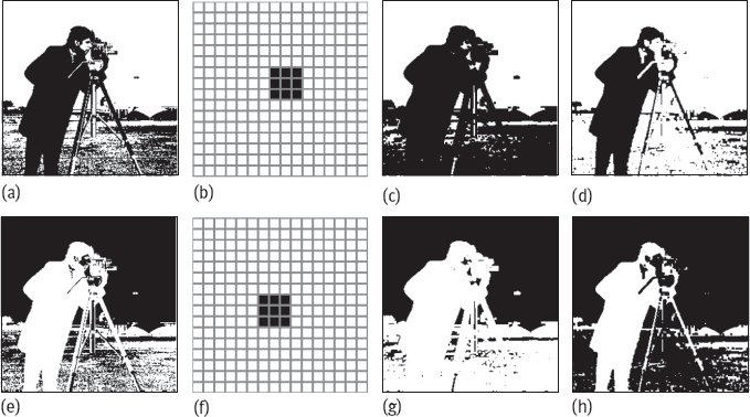
A set of real images corresponding to Figure 8.5 are shown in Figure 8.6, in which the duality of dilation and erosion is further verified. Figure 8.6(a) is a binary image obtained by thresholding Figure 1.1(b). ![]()
8.1.2Binary Opening and Closing
Opening and closing can also be considered as one basic pair of binary morphology operations.
8.1.2.1Definitions
Dilation and erosion are not the inverse of each other, so they can be cascaded in combination. For example, the image may be first eroded and then the result dilated, or the image may be first dilated and then the result eroded (using the same structure elements). The former operation is called opening and the latter operation is called closing. They are also important mathematical morphology operations.
The operator for opening is ○, opening A by B is written A ○ B and is defined as:
The operator for closing is ●, closing A by B is written A● B, and is defined as:
Both opening and closing are operations that can remove specific image details smaller than structure elements, while ensuring no global geometric distortion. Opening operation can filter off spines smaller than structure elements, cut out the elongated lap and play the role of separation. Closing operation can fill notches or holes smaller than structure elements and play the role of connection.
The ability of opening and closing for extracting shape matched to the structure elements in image can be obtained by the following characteristic theorems for opening and closing, respectively:
Equation (8.13) shows that opening A by B is to select some points in A and matched to B, these points can be completely obtained by the structure element B contained in A. Equation (8.14) shows that the result of closing A by B includes all points met the following conditions, that is, when the point is covered by the mapped and shifted structure elements, the intersection of A and the mapped and shifted structure elements is not zero.
8.1.2.2Geometric Interpretation
Opening and closing can be given simple geometric interpretation by combining the method of the set theory. For opening, the structure element can be considered as a ball (on plane), the result of opening is outer edge of the ball rolling inside the set to be opened. Based on the filling property of opening operation, an implementation method based on set theory can be obtained. That is, opening A by B can be achieved by combining all results of filling B in A and then shift and compute their union. In other words, opening can be described using the following filling process:
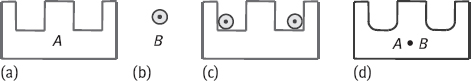
One example is given in Figure 8.7, in which Figure 8.7(a) gives A, Figure 8.7(b) gives B, Figure 8.7(c) shows B in several locations of A, Figure 8.7(d) gives the result of opening A by B.
There is a similar geometric interpretation for closing, the difference is now the structure elements are considered in the background. One example is given in Figure 8.8, in which Figure 8.8(a) gives A, Figure 8.8(b) gives B, Figure 8.8(c) shows B in several positions in A, Figure 8.8(d) gives the result of closing A by B.
8.1.2.3Duality of Binary Opening and Closing
Similar to dilation and erosion, opening and closing also have duality. The duality of opening and closing can be expressed as
This duality can be derived from the duality of dilation and erosion represented by eqs. (8.9) and (8.10).
8.1.2.4Relationship Between the Set and Binary Opening and Closing
The relationship between the set as well as binary opening and closings can be represented by four swap properties listed in Tables 8.1.
When the objects of operation are multiple images, the opening and closing can be performed with the help of the property of sets:
1.Opening and union: the opening of union includes the union of opening;
2.Opening and intersection: the opening of intersection is included in the intersection of opening;
3.Closing and union: the closing of union includes the union of closing;
4.Closing and intersection: the closing of intersection is included in the intersection of closing.
Example 8.8 Comparative examples of four basic operations.
A group of results obtained by using the four basic operations for a same image are presented in Figure 8.9 for comparison. The image A is shown in Figure 8.9(a). The structure element consists of the origin point and its 4-neighbors. From Figure 8.9(b, e), the results obtained by using dilation, erosion, opening, and closing are given, respectively. Wherein, the dark pixels in Figure 8.9(b) are expanded pixels, the dark pixels in Figure 8.9(d) are pixels of first eroded and then expanded, and the dark pixels in Figure 8.9(e) are those pixels first expanded out but not eroded after then. It is clear there exists A ⊖ B ⊂ A ⊂ A ⊕ B. In addition, the opening operation achieves the goal of producing a more compact and smooth contour of the object by eliminating the spike (or narrow band) on the object; while the closing operation realizes the filling of depressions (or holes) on the object. Both operations reduced the irregular nature of the contour. ![]()
8.2Combined Operations of Binary Morphology
Four basic operations of binary mathematical morphology (dilation, erosion, opening, and closing) have been introduced in the previous section. Someone regarded the hit-or-miss transform as also a basic operation of binary mathematical morphology. If the hit-or-miss transform is combined with the above four basic operations, some other composition operations and fundamental algorithms for morphological analysis can be obtained.
8.2.1Hit-or-Miss Transform
The hit-or-miss transform (or hit-or-miss operator) in mathematical morphology is a basic tool for shape detection and is also the basis for many composition operations. Hit-or-miss transform actually corresponds to two operations, so it uses two structure elements. Let A be the original image, E and F are a pair of non-overlapping set (which define a pair of structure elements). Hit-or-miss transform is represented by ⇑ and is defined as:
In the result of hit-or-miss transform, any pixel z meets E + z is a subset of A, and F + z is a subset of Ac. Conversely, the pixel z met the two conditions must be in hit-or-miss transform results. E and F are called hit structure element and miss structure element, respectively. Figure 8.10(a) is the hit structure element. Figure 8.10(b) is the miss structure element. Figure 8.10(c) gives four examples of the original images. Figure 8.10(d) provides the results obtained by using hit-or-miss transform, respectively. Note that two structure elements need to meet E ∩ F = ∅; otherwise, the hit-or-miss transform will produce empty set.
Example 8.9 Hit-or-miss transform examples.
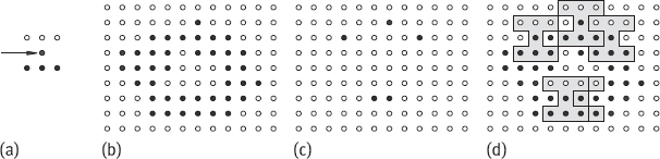
In Figure 8.11, ● and ○ represent the object and the background pixels, respectively. Let structure element B be as shown in Figure 8.11(a), the arrow points to the pixel corresponding to center (origin) of B. If the object A is as shown in Figure 8.11(b), then the result of A ⇑ B is shown in Figure 8.11(c). Figure 8.11(d) provides further explanation, the object pixels remained in the result of A ⇑ B correspond to the pixels whose neighborhood in A matches to structure element B. ![]()

8.2.2Binary Composition Operations
Composition operations combine the basic operations to complete some meaningful actions, or to achieve some specific image processing functions.
8.2.2.1Convex Hull
The convex hull of a region is one of presentation means for this region (Section 3.2.3). Given a set A, it is possible to use a simple morphology algorithm to get its convex hull H(A). Let Bi, i = 1, 2, 3, 4, be four structure elements, first constructing
In the above equation, Let now where the superscript “conv” indicates the convergence at the sense of According to these definitions, the convex hull of A can be expressed as
In other words, the construction process for convex hull is as follows. First, performing iteratively hit-or-miss transform to the region A with B1, when no further changes will be evaluated, the union of the transform result and A is computed, this union result is noted as D1. Then, B2 is used for transform, repeating iteration and seeking union, the union result is recorded as D2. This procedure will be conducted also for B3 and B4 to obtain the D3 and D4; the union of four results D1, D2, D3, and D4 provides the convex hull of A.
Example 8.10 Construction of convex hull.
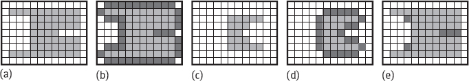
One example of constructing convex hull is presented in Figure 8.12. Figure 8.12(a) gives the four structure elements used, the origin of each structure element is in the center, “×” means it can be any value. Figure 8.12(b) shows the set A whose convex hull needs to construct. Figure 8.12(c) is the result obtained by starting from and after four iterations according to eq. (8.19). Figure 8.12(d–f) are the results obtained by starting from and after two iterations, eight iterations, two iterations according to eq. (8.19), respectively. The finally obtained convex hull is the union of the above four results according to eq. (8.20), as shown in Figure 8.12(g). In Figure 8.12(h), the numbers indicate the contribution of different structure elements in constructing the convex hull. ![]()

8.2.2.2Thinning
In some applications (such as seeking skeleton), it is hoped to erode the object region but do not to split it into multiple subregions. Here, the pixels located around the boundary of the object region are to be checked, to see whether they can be removed without splitting the object region into multiple sub-regions. This task can be achieved by thinning. Thinning set A by structure element B is noted as A ⊗ B, which can be defined (with the help of hit-or-miss transform) as follows:
In the above equation, hit-or-miss transform is used to determine the pixels that should be thinning out, then they can be removed from the original set A. In practice, a series of masks with small size are used. If a series of structure element is defined as {B} = {B1, B2, ..., Bn}, in which Bi+1 represents the result of rotating Bi, then thinning can be defined as:
In other words, this process is first using B1 for thinning A, then using B2 for thinning the previous result, and so on until Bn is used for thinning. The whole process can be repeated until no change produced so far.
The following set of four structure elements (hit-or-miss masks) can be used for thinning (“×” denotes the value 0 or 1):
Example 8.11 A thinning process and results.
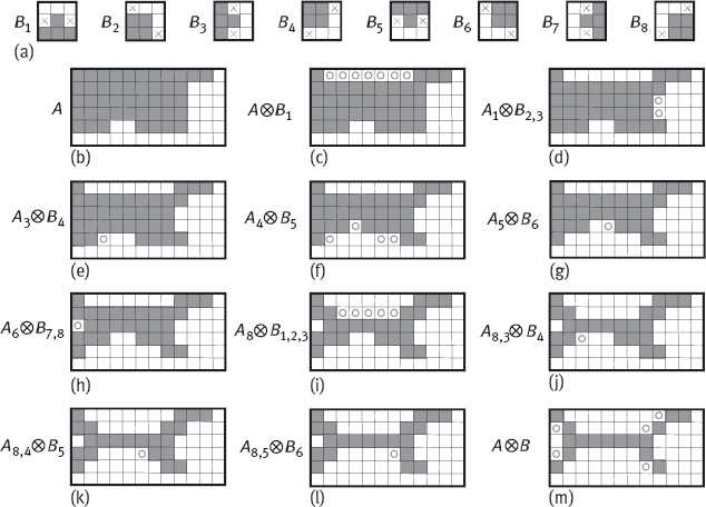
A set of structure elements and a thinning process using these structure elements are presented in Figure 8.13. Figure 8.13(a) gives a set of structure elements commonly used, in which the origin of a structure element is in its center, white and gray pixels have values 0 and 1, respectively. If the points detected by structure element B1 are subtracted from the object, the object will be thinned from the upper side, if the points detected by structure element B2 are subtracted from the object, the object will be thinned from the upper right corner, and so on. With the above set of structure elements, symmetrical thinning results will be obtained. Besides, the four structure elements with odd numbers have stronger thinning capability, while the four structure elements with even numbers have weaker thinning capability.
Figure 8.13(b) shows the original region to be thinned, its origin is located in the upper left corner. Figure 8.13(c, k) provides successively the thinning results with the various structure elements (circles mark the pixels thinned out in the current step). The converged result obtained by using B6 a second time is shown in Figure 8.13(l). Final result obtained by converting the thinning result to a mixed connectivity to eliminate multi-connection problem is shown in Figure 8.13(m). In many applications (such as seeking skeleton), it is required to erode the object but does not to break the object into several parts. To do this, a number of points on the contour of the object should be first detected. Removing these points will not lead the division of object into two parts. Using the above hit-or-miss masks can satisfy this condition.
![]()
8.2.2.3Thickening
Thickening set A by structure element B is denoted by From the point of morphological view, thickening corresponds to thinning, and can be defined by
Similar to thinning, thickening can also be defined by a series of operations:
The structure elements used in thickening are similar as in thinning, only 1 and 0 should be exchanged over. In practice, the thickening results are often obtained by first thinning background and then finding the complements of thinning results. In other words, if a set A needs to be thickened, it can be achieved by first constructing C = Ac, then thinning C, and finally seeking Cc.
Example 8.12 Using thinning for thickening.
One example of using thinning for thickening is given in Figure 8.14. Figure 8.14(a) is the set A. Figure 8.14(b) is C = Ac. Figure 8.14(c) shows the result of thinning. Figure 8.14(d) shows the Cc obtained from the complement Figure 8.14(c), and the thickening result after simple post-treatment for removing disconnected points is shown in Figure 8.14(e). ![]()
8.2.2.4Pruning
Pruning is an important complement to thinning and skeleton extraction operation, or it is often used as a post processing means for thinning and skeleton extraction. Because the thinning and skeleton extraction often leave some excessive parasitic components, so it is necessary to use a method such as pruning as postprocessing to eliminate these components. Pruning can make use of a combination of several methods above to achieve. To explain the pruning process, let us considering an example of handwritten character recognition using automatic methods, as shown in Figure 8.15. A skeleton for a handwritten character “a” is given in Figure 8.15(a). The segment at the leftmost of the character is a typical example of a parasitic component. To solve this problem, it is possible to continuously eliminate the endpoint. Of cause, this process will eliminate or shorten other segments in the character. It is assumed that the length of the parasitic segment is not more than three pixels, so the process is designed to eliminate only segments with less than three pixels. For a set A, using a series of structure elements capable of detecting endpoint to thin A can get the desired results. Let
where {B} represent the structure elements series, as shown in Figure 8.15(b, c). This series contains two kinds of structures, rotating each series can obtain four structure elements, so there are a total of eight structure elements.

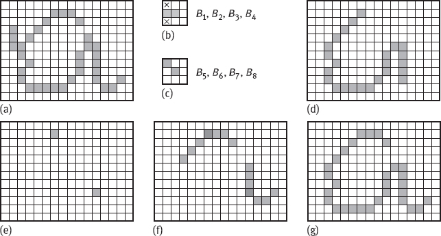
Thinning set A three times, according to eq. (8.26), gives the result X1 as shown in Figure 8.15(d). The next step is to restore the character to get the original shape without the parasitic segment. To do this, a set X2 with all endpoints of X1 is constructed, as shown in Figure 8.15(e).
wherein Bk is an endpoint detector. In the following, dilating endpoints three times by taking A as constrain to obtain X3:
wherein H is a 3 × 3 structure element with all pixel values 1. Such a conditional dilation can prevent to produce value 1 elements outside of the region of interest, as shown in Figure 8.15(f). Finally, the union of X1 and X3 provides the result shown in Figure 8.15(g).
The above pruning process cyclically uses a set of structure elements for eliminating noise pixels. Generally, an algorithm only uses one or two cycles of this set of structure elements; otherwise, it is possible that the object region in image may be undesirably changed.