8.3.1Noise Removal

The binary image obtained by segmentation often consists of some small holes or islands. These holes or islands are generally caused by the system noise, threshold value selected or preprocessing. Pepper and salt noise is a typical noise, which leads to small holes or islands in binary images. Combining the opening and closing operations could constitute a noise filter to eliminate this type of noise. For example, using a structure element comprising a central pixel and its 4-neighborhood pixels for the opening of the image can eliminate the pepper noise, while using this structure element for the closing of the image can eliminate the salt noise (Ritter 2001).

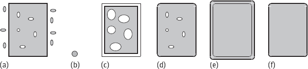
One example of noise removal using a combination of opening and closing is given in Figure 8.16. Figure 8.16(a) comprises a rectangular object A, due to the influence of noise, there are some holes inside of the object and some blocks around the object. Now, the structure elements B, as shown in Figure 8.16(b), will be used by morphological operations to eliminate noise. Here, the structure element should be larger than all of the holes and blocks. The first step is to erode A by B, which gives Figure 8.16(c). The second step is to dilate Figure 8.16(c) by B, which gives Figure 8.16(d). The serial combination of erosion and dilation operations is an opening operation, it will eliminate the noise around the object. Now, Figure 8.16(d) is dilated by B, which gives Figure 8.16(e). Finally, Figure 8.16(e) is eroded by B, which gives Figure 8.16(f). The serial combination of these last two operations is a closing operation, the noise inside the object will be eliminated. The whole process is first opening and then closing, it can be written as

$\left\{\left[A\right]\right\}\ominus B)\oplus B]\oplus B\}\ominus B=(A\circ B)•B(8.30)$

Comparing Figure 8.16(a, f), it is seen that the inside and outside noises are both eliminated, while the object itself has not been changed much, except that the original four right angles turn to be rounded.

8.3.2Corner Detection

Corner pixel is located at the place where the slope has a sudden change and the absolutely curvature is very big. Corner pixel can be extracted by means of morphological operations. In the first step, a circular structure element with a suitable size should be selected, using the structure element for opening and subtract the result from the original image. Then two new structure elements are selected, one is bigger than the remaining area, another is smaller than the remaining area. Using these two structure elements to erode the remaining area, and comparing the two results obtained. This is equivalent to a band-pass filter.

Corner detection can also be achieved by means of asymmetric closing (Shih 2010). Asymmetrical closing comprises two steps. First a structure element is used to dilate the image, then another structure element is used to erode the image. The idea is to make dilation and erosion complementary. For example, two structure elements with forms of cross “+” and diamond “◊” can be used. The asymmetric closing for image A can be expressed by the following equation:

$A_{+◇}^c=(A\oplus +)\ominus ◇(8.31)$

Here, the corner strength is

$C_{+}(A)=\left|A-A_{+◇}^c\right|(8.32)$

For different corner points, the corner strength after rotating 45° can also be calculated (the structure elements are square □ and cross ×, respectively):

$C_{\times }(A)=\left|A-A_{\times \square }^c\right|(8.33)$

The above four structure elements can be combined (in sequence as shown in Figure 8.17), then the detection of the corners can be written as

$C_{+\times }(A)=\left|A_{+◇}^c-A_{+◇}^c\right|(8.34)$

8.3.3Boundary Extraction

Suppose there is a set A, its boundary is denoted by β(A). By first eroding A by a structure element B and then taking the difference between the result of erosion and A, β(A) can be obtained:

$\beta (A)=A-(A\ominus B)(8.35)$

Let us look at Figure 8.18, wherein Figure 8.18(a) is a binary object A, Figure 8.18(b) is a structure element B, Figure 8.18(c) shows the result of eroding A by B, A ⊖ B, Figure 8.18(d) is the final result obtained by subtracting Figure 8.18(c) from Figure 8.18(a). Note that when the origin of B is at the edge of A, some parts of B will be outside A, where is generally set to 0. Also note that the structure element is 8-connected, while the resulting border is 4-connected.

8.3.4Object Detection and Localization

How to use hit-or-miss transform to determine the location of a given size square (object) is explained with the help of Figure 8.19 (Ritter, 2001). Figure 8.19(a) is the original image, including four solid squares of size 3 × 3, 5 × 5, 7 × 7, and 9 × 9, respectively. Taking the 3 × 3 solid square in Figure 8.19(b) as a structure element E, and the 9 × 9 box frame (edge width of one pixel) in Figure 8.19(c) as another structure element F. Their combination constitute a pair of structure elements B = (E, F). In this example, the hit-or-miss transform E is designed to hit region covered by E and to miss the region covered by F. The finally obtained results are shown in Figure 8.19(d).

8.3.5Region Filling

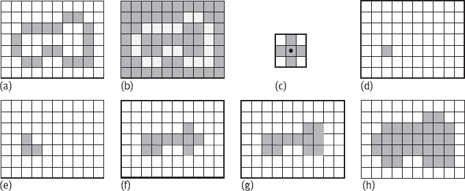
A region and its boundary can be mutually demanded. When a region is known, its boundary can be obtained according to eq. (8.35). On the other side, when a boundary is known, the region can be obtained by region filling.An example is given in Figure 8.20, wherein Figure 8.20(a) provides boundary points for a region A, its complement is given in Figure 8.20(b). The region A can be filled by using the structure element in Figure 8.20(c) for computing dilation, complement, and intersection. First, assigning 1 to a point within the boundary (as shown by the dark pixel in Figure 8.20(d)), then filling the inside of the boundary according to the following iterative equation (Figure 8.20(e, f) provides the situations in two intermediate steps, respectively)

$X_k=\left(X_{k-1}\oplus B\right)\cap A^c,k=1,2,3,\mathrm{...}(8.36)$

The iteration will be stopped when Xk = Xk–1 (in this example k = 7, as shown in Figure 8.20(g)). At this moment, the intersection of Xk and A includes the inside and boundary of filled region, as shown in Figure 8.20(h). The dilation process in eq. (8.36) must be controlled to avoid exceeding the boundary, but the computation of intersection with Ac at every step will limit it in the region of interest. This dilation process can be called a conditional dilation process. Note that the structure element here is 4-connected, while the original filled boundary is 8-connected.

8.3.6Extraction of Connected Components

Let Y represent a connected component in a set A, and one point in Y is known, then all the elements in Y can be obtained by using the following iterative formula:

$X_k=\left(X_{k-1}\oplus B\right)\cap A,k=1,2,3,\mathrm{....}(8.37)$

When Xk = Xk–1, stop iteration, then Y = Xk.

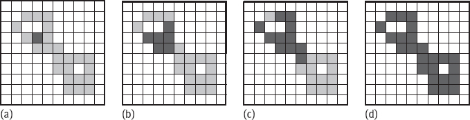
Comparing eqs. (8.37)–(8.36), except replacing Ac by A, they are identical. Because here the elements needed to extract have been marked as 1. Computing intersection with A in each iteration can remove the dilation taking the element marked 0 as the center. One example of extraction of connected components is shown in Figure 8.21, where the structure element used is same as in Figure 8.20. In Figure 8.21(a), the values of lightly shaded pixels (i. e., the connected components) are 1, but at this time, these pixels have not yet been discovered by algorithm. The values of darkly shaded pixels in Figure 8.21(a) are also 1 and that they are known to belong Y. These pixels can be taken as the start points of algorithm. The results of first and second iterations are given in Figure 8.21(b, c), respectively. The final result is given in Figure 8.21(d).

8.3.7Calculation of Region Skeleton

In Section 3.3.5, the concept of the skeleton and a computational method are introduced. Here, a technique for calculating skeleton with mathematical morphological operations is presented. Let S(A) represent the skeleton of A, which can be expressed as

$S(A)={\displaystyle \underset{k=0}{\overset{K}{\cup }}{S}_k(A)(8.38)}$

The Sk(A) in the above formula is generally referred to as a subset of the skeleton, which can be written as

$S_k(A)=(A\ominus kB)-[(A-\ominus kB)\circ B](8.39)$

where B is a structure element; (A ⊖ kB) means eroding A by B for k consecutive times, which can be represented by Tk:

$T_k=(A\ominus kB)=((\mathrm{...}(A\ominus B)\ominus B)\ominus \mathrm{....})\ominus B(8.40)$

K in eq. (8.38) represents the last iteration in eroding A to the empty set, namely

$K=\max \left\{k\right|(A\ominus kB)\ne \cancel{0}\}(8.41)$

Example 8.13 Morphological skeleton.

One example of computing the skeleton with morphological operations is shown in Figure 8.22. In the original image (top left), there is a rectangular object that has a little addenda above it. The first row then shows the result sets Tk obtained by sequentially erosions, i. e., T0, T1, T2, T3, T4. Because T4 = ∅, so K = 3. The second line gives a set of sequentially obtained skeleton sets Sk, that is, S0, S1, S2, S3, and the final skeleton S (including two separately connected portions).

Equation (8.38) shows that the skeleton A may be obtained by the union of a subset Sk(A). Conversely, A can also be used for the reconstruction of Sk(A):

$A={\displaystyle \underset{k=0}{\overset{k}{\cup }}\left(S_k\left(A\right)\oplus kB\right)}\left(8.42\right)$

wherein B is a structure element; (Sk(A) ⊕ kB) represents the dilation of Sk(A) by B for k consecutive times, namely

$\left(s_k\left(A\right)\oplus kB\right)=\left(\left(\cdot \cdot \cdot \left(s_k\left(A\right)\oplus B\right)\oplus B\right)\oplus \cdot \cdot \cdot \right)\oplus B\left(8.43\right)$

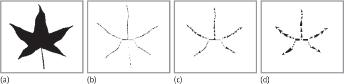
Example 8.14 A real example of morphological skeleton.

One example of computing the skeleton of a real image is shown in Figure 8.23. Figure 8.23(a) is a binary image; Figure 8.23(b) shows the skeleton obtained using the structure element of 3 × 3 in Figure 8.18; Figure 8.23(c) shows the skeleton obtained using a similar structure element of 5 × 5; and Figure 8.23(d) shows the skeleton obtained using a similar structure element of 7 × 7. Note that in Figure 8.23(c, d), since the masks are relatively big so the petiole is not preserved.

8.4.1Grayscale Dilation and Erosion

Grayscale dilation and erosion are the most basic operations of grayscale mathematical morphology. Different from the binary dilation and erosion operations, in which the result is mainly reflected in the image plane, the result of grayscale dilation and erosion operations is mainly reflected in the amplitude axis.

8.4.1.1Grayscale Dilation

The grayscale dilation of input image f by structure element b is denoted by f ⊕ b, which is defined as

$\left(f\oplus b\right)\left(s,t\right)=\max \left\{f\left(x,y\right)+b\left(s-x,t-y\right)|\left(x,y\right)\in D_f\text{and}\left[\left(s-x\right),\left(t-y\right)\right]\in D_b\right\}\left(8.44\right)$

where Df and Db are the domains of definition of f and b, respectively. Here, limiting [(s – x), (t – y)] inside the domain of definition of b is similar to the binary dilation in which at least two elements from each of two operands have a (nonzero) element in intersection. Equation (8.44) is very similar to the formula of 2-D convolution, the differences here are that the max (maximum) has replaced the summation (or integration) in convolution and the addition has replaced the multiplication in convolution. In the dilated grayscale images, the region that is brighter than the background will be expanded, while the region that is darker than the background will be condensed.

In the following, the meaning and operation mechanism of operation in eq. (8.44) are first briefly explained with 1-D function. When considering the 1-D function, eq. (8.44) is simplified to:

$\left(f\oplus b\right)\left(s\right)=\max \{f\left(x\right)+b\left(s-x\right)|x\in D_f\text{and}\left(s-x\right)\in D_b\left(8.45\right)$

Similar as in convolution, b(–x) is the inverted mapping of b(x) respective to the origin of x-axis. For positive s, b(s – x) moves to the right; for negative s, b(s – x) moves to the left. The requirements of x in the domain of definition of f and of (s – x) values in the domain of definition of b is to make f and b coincide.

Example 8.15 Illustration of grayscale dilation.

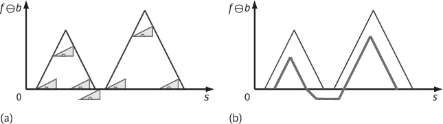
An illustration of grayscale dilation is shown in Figure 8.24. Figure 8.24(a, b) gives f and b, respectively. In Figure 8.24(c), several locations of the structure element (inverted) during the calculation process are provided. In Figure 8.24(d), the bold line gives the final dilation results. Due to the interchangeable property of dilation, if let f have reverse translation for dilation, it will produce exactly the same result.

The computation of dilation is to select the maximum value of f + b in the neighborhood determined by the structure element. Therefore, there will be two effects with the dilation of gray-scale images:

1.If the values of the structure element are all positive, then the output image will be brighter than the input image.

2.If the size of dark details in input image is smaller than the structure element, then the visual effect will be weakened. The degree of diminished extent depends on the gray-level values surrounding these dark details and the shape and magnitude values of structure elements.

Example 8.16 The numerical computation of grayscale dilation.

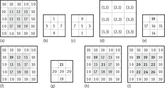
One example for the computation of grayscale dilation is shown in Figure 8.25. Figure 8.25(a) is a 5 × 5 image A. Figure 8.25(b) is a 3 × 3 structure element B with its origin at the center. Figure 8.25(c) is its inversion. Since the size of B is 3 × 3, in order to avoid the coefficient of B falling out of A upon dilation, the edge pixels of A will not be considered, that is, for a 5 × 5 image A, considering only the 3 × 3 center portion. The origin of A, (0, 0), is at the upper left corner, so the coordinates of 3 × 3 center portion are shown as in Figure 8.25(d). If overlapping the origin of B with (1, 1) in image A, and calculating the sum of each value of B with its corresponding pixel value in A, the result is shown in Figure 8.25(e). Taking the highest value as the result of dilation, the A will be updated as shown in Figure 8.25(f). Another example, overlapping the origin of B with (2, 2) and also calculating the sum of each value of B with its corresponding pixel value in A, the results is shown in Figure 8.25(g). Then, taking the highest value as the result of dilation, the A will be updated again as shown in Figure 8.25(h). Dilating all center 3 × 3 pixels of A as above, the final result is shown in Figure 8.25(i). a

8.4.1.2Grayscale Erosion

The grayscale erosion of input image f by structure element b is denoted by f ⊖ b, which is defined as

$\left(f\oplus b\right)\left(s,t\right)=\max \left\{f\left(x,y\right)+b\left(s+x,t+y\right)|\left(x,y\right)\in D_f\text{and}\left(s+x,\left(t+y\right)\right)\in D_b\right\}\left(8.46\right)$

where Df and Db are the domains of definition of f and b, respectively. Here, limiting [(s – x), (t – y)] in the domain of definition of b is similar to in the definition of binary erosion in which the structure elements are required to be included completely in eroded set. Equation (8.46) is very similar to 2-D correlation, except that here the summation (or integration) in correlation is replaced by the min (minimum) operation, and the multiplication in correlation is replaced by subtraction. Therefore, in the results of grayscale image erosion, the region that is darker than the background will be expanded and the region that is brighter than the background will be condensed.

For simplicity, similar as in the discussion of the dilation, the meaning and operation mechanism of operation in eq. (8.46) are first briefly explained with 1-D function. When considering the 1-D function, eq. (8.46) can be simplified to

$(f\ominus b)(s)=\min \{f(x)-b(s+x)|x\in D_{f}and(s+x)\in D_b\}(8.47)$

Similar as in convolution, for positive s, b(s + x) moves to the right; for negative s, b(s + x) moves to the left. The requirements of x in the domain of definition of f and of (s + x) in the domain of definition of b are to make b totally be contained in the definition range of f.

Example 8.17 Illustration of grayscale erosion.

An illustration of grayscale erosion is shown in Figure 8.26. The input image f and the structure element b are the same as in Figure 8.24. Figure 8.26(a, b) provides several locations of the structure element (b shifted) and the final result of erosion, respectively.

The computation of erosion is to select the minimum value of f – b in the neighborhood determined by the structure element. Therefore, there will be two effects with the erosion of grayscale images:

1.If the values of the structure element are all positive, then the output image will be darker than the input image.

2.If the size of light details in input image is smaller than the structure element, then the visual effect will be weakened. The degree of diminished extent depends on the gray-level values surrounding these light details and the shape and magnitude values of structure elements.

Example 8.18 The numerical computation of grayscale erosion.

One example for the computation of grayscale erosion is shown in Figure 8.27. The images A and structure element B used are still the same as in Figure 8.25. Similar to Example 8.16, if overlapping the origin of B with (1, 1), and calculating the sum of each value of B with its corresponding pixel value in A, the result is shown in Figure 8.27(a). Taking the smallest value as the result of erosion, the image A will be updated as shown in Figure 8.27(b). If overlapping the origin of B with (2, 2) and also calculating the sum of each value of B with its corresponding pixel value in A, the results is shown in Figure 8.27(c). Then, taking the lowest value as the result of erosion, the A will be updated again as shown in Figure 8.27(d). Eroding all center 3 × 3 pixels of A as above, the final result is shown in Figure 8.27(e).

Example 8.19 Grayscale dilation and erosion.

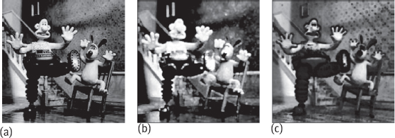
One example of grayscale dilation and erosion is shown in Figure 8.28. Figure 8.28(a) is the original image. Figure 8.28(b, c) are the results obtained by one dilation and one erosion, respectively. The value at the center of structure elements is 2, the four neighborhood pixels have values 1.

8.4.2Grayscale Opening and Closing

The representations of opening and closing in grayscale mathematical morphology are consistent with their corresponding operations in binary mathematical morphology. Opening f by b is denoted as f ○ b, which is defined as

$f\circ b=(f\ominus b)\oplus b(8.50)$

Closing f by b is denoted as f ● b, which is defined as

$f•b=(f\oplus b)\ominus b(8.51)$

Opening and closing are dual with the complement of function and reflector of function, their duality can be expressed as

${(f\circ b)}^c=f^c•\widehat{b}(8.52)$

${(f•b)}^c=f^c\circ \widehat{b}(8.53)$

Since fc(x, y) = –f(x, y), eqs. (8.52) and (8.53) can also be written as

$-(f\circ b)=-f•\widehat{b}(8.54)$

$-\left(f•b\right)=-f\circ \widehat{b}(8.55)$

Example 8.20 Grayscale opening and closing.

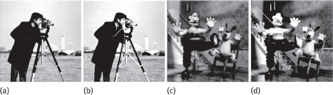
Some results obtained by using grayscale mathematical morphology operations are shown in Figure 8.29. Figure 8.29(a, b) is results of grayscale opening and grayscale closing operations, respectively. The grayscale structure elements used are the same as in Example 8.19. Note that in Figure 8.29(a) the operating handle held by photographer is now less obvious, which indicates the operation of grayscale opening eliminated smaller bright details. On the other hand, the blur of photographer’s mouth shows that grayscale closing can eliminate smaller dark details. Figure 8.29(c, d) shows the results of grayscale opening and grayscale closing of Figure 8.28, respectively. The grayscale opening make the image to become darker, while the grayscale closing make the image to become brighter.

8.5.1Morphological Gradient

Dilation and erosion are often combined for computing morphological gradient. The morphological gradient of an image is denoted g:

$g=(f\oplus b)-(f\ominus b)(8.56)$

Morphological gradient can enhance relatively sharp transition region in the gray-level image. Different from a variety of spatial gradient operators (Section 2.2.1), the morphological gradient obtained by using symmetrical structure elements is less affected by the edge direction, but the amount of computation required for computing morphological gradient is generally large.

Example 8.21 Result of morphological gradient calculation.

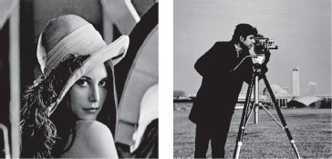
Some gradient calculation results are given in Figure 8.30. Figure 8.30(a, b) is the results of morphological gradient calculated for the two images in Figure 1.1. For comparison, Figure 8.30(c) shows the (amplitude) result of using Sobel gradient operator for the second image.

8.5.2Morphological Smoothing

One kind of image smoothing methods can be achieved by first opening and then closing. Suppose the result of morphological smoothing is g:

$g=\left(f\circ b\right)•b\left(8.57\right)$

The combined effect of the two operations is to remove or reduce all kinds of noise in the relative lighter and darker regions, in which the opening can remove or reduce the noise in lighter region that is smaller in size than the structure elements, while the closing can remove or reduce the noise in darker region that is smaller in size than the structure elements.

Example 8.22 Morphological smoothing.

The result of morphological smoothing for image in Figure 1.1(b) is shown in Figure 8.31, here a grayscale structure element using four neighborhood is taken. After smoothing, the ripple on the tripod has been removed, and the image appears more smoothing.

8.5.3Top Hat Transform and Bottom Hat Transform

Top hat transform gets the name from the structure element it used, which is a cylinder or parallelepiped with the flat upper portion (like a hat). The results of top hat transforming an image f with a structure element b is noted as Th:

$T_{\text{h}}=f-\left(f\circ b\right)\left(8.58\right)$

The process is to subtract the result of opening an original image from the original image itself. This transform is suitable for images with bright target on a dark background, which can enhance image detail in the bright region.

The corresponding transform of top hat transform is bottom hat transform. From its name, it is clear that the structure element used should be a cylinder or parallelepiped with the flat bottom portion (like a hat upside down). In practice, the cylinder or parallelepiped with the flat upper portion can still be used as structure elements, but the operation instead will be first using structural element for closing the original image, and then subtracting the original image from the result. The results of bottom hat transforming an image f with a structure element b is noted as Tb:

$T_{\text{b}}=\left(f•b\right)-f\left(8.59\right)$

This transformation applies to image with dark target on a light background, the image details in the dark region can be enhanced.

Example 8.23 Top hat transform examples.

Using the grayscale structure elements with 8-neighborhood as top hats, and applying them to the two images in Figure 1.1 can provide the top hat transform results as shown in Figure 8.32.

8.5.4Morphological Filters

Morphological filter is a group of nonlinear signal filters using morphological transformations to locally modify the geometric characteristics of the signal (Mahdavieh, 1992). If each signal in Euclidean space is seen as a set, then the morphological filtering is the signal set operations to change the shape of signal. Given filtering operation and the filter output, a quantitative description of the geometry of the input signal can be obtained.

Dilation and erosion are not the inverse of each other, so their applying order cannot be interchanged. For example, the discarded information during erosion process cannot be recovered by dilating the erosion result. Among the basic morphological operations, dilation and erosion are rarely used alone. By combining dilation and erosion, the opening and closing can be formed, their various combinations are the most commonly used in the image analysis. One implementation of morphological filters is to combine opening and closing together. Opening and closing can be used for the quantitative study of the geometric characteristics, because they have little effect on the retention or removal of grayscale features.

From the point of view to eliminate the structures that is brighter than the background and that is smaller than the structure elements, the opening operation is roughly like nonlinear low-pass filter. However, the opening is different from low-pass filtering that prevents a variety of high-frequency components in the frequency domain. In case when both big and small structures have high frequency, the opening allows to pass only large structures but to remove small structures. Opening an image will eliminate bright dots in the image, such as island or spike. Closing has the corresponding functions on darker features as the opening has on lighter features, it can remove those structure that is darker than the background and whose size is smaller than the structure elements.

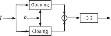
The combination of opening and closing can be used to eliminate noise. If a small structure element is used to first open and then close an image, it is possible to remove from image the noise-like structures whose size are smaller than the structure elements. A commonly used structure element is a small hemisphere. The diagram of a hybrid filter is shown in Figure 8.33. It should be noted, in filtering noise, the median, Sigma and Kalman filter are often better than mixed morphological filters.

Sieve filter is a morphological filter that allows only structures within a narrow size range passing through. For example, to extract the light defects with size of n × n pixels (n is an odd number), the following filter S (superscript denotes the size of structure elements) can be used:

$S=\left(f\circ b^{n\times n}\right)-\left[f\circ b^{\left(n-2\right)\times \left(n-2\right)}\right]\left(8.60\right)$

Sieve filter is similar to the band-pass filter in frequency domain. In the above formula, the first term can remove all light structures with size smaller than n × n, the second term can remove all light structures with size smaller than (n – 2) × (n – 2). The subtraction of two terms leaves the structures between n × n and the (n – 2) × (n – 2).

8.5.5Soft Morphological Filters

Soft morphological filters and basic morphological filter are very similar, the main difference is that soft morphological filter is not very sensitive to additive noise and to the shape changes of object to be filtered.

Soft morphological filters can be defined on the basis of weighted-order statistics. Two basic morphological filtering operations are soft erosion and soft dilation. It is required to replace the standard structure elements by the structuring systems. A structural system including three parameters is denoted as [B, C, r]: B and C are finite plane sets, C ⊂ B, r is a natural number satisfying 1 ≤ r ≤ |B|. Set B is called a structure set, C is its hard center, B – C gives its soft contours, and r is the order of the center. Soft morphological filter can convert a gray-level image f(x, y) into another image.

Using the structuring system [B, C, r] to soft dilate f(x, y) is denoted as f ⊕ [B, C, r](x, y), which is defined as:

$f\oplus \left[B,C,r\right]\left(x,y\right)=r\text{th}\text{Max}\text{of}\left\{r\diamond f\left(c\right):c\in C_{\left(x,y\right)}\right\}\cup \left\{f\left(b\right):b\in {\left(B-C\right)}_{\left(x,y\right)}\right\}\left(8.61\right)$

where ◊ represents a repeating operation, the part in braces is a multiset that is a set of objects on which the operation can be repeated. For example, {1, 1, 1, 2, 3, 3} = {3 ◊ 1, 2, 2 ◊ 3}} is a multiset.

Using the structuring system [B, C, r] to soft erode f(x, y) is denoted as f ⊖ [B, C, r](x, y), which is defined as:

$f\ominus \left[B,C,r\right]\left(x,y\right)=r\text{th}\text{Max}\text{of}\left\{r\diamond f\left(c\right):c\in C_{\left(x,y\right)}\right\}\cup \left\{f\left(b\right):b\in {\left(B-C\right)}_{\left(x,y\right)}\right\}\left(8.62\right)$

Using the structuring system [B, C, r] to soft dilate or soft erode f(x, y) at position (x, y) needs to move B and C to (x, y) and to form multiset with values of f(x, y) inside the moved sets. Wherein the values of f(x, y) at the hard center need to repeat first r times, then for soft dilation the rth maximum value from the multiset is taken while for soft erosion the rth minimum value from the multiset is taken.

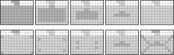
One example of soft dilation is given in Figure 8.34. Figure 8.34(a) shows the structure element B and its center C, in which light points represent the origin of coordinate system and also C (an element of B), and dark points represent elements belong to B. Figure 8.34(b) is the original image. Figure 8.34(c) shows f ⊕ [B, C, 1]. Figure 8.34(d) shows f ⊕ [B, C, 2]. Figure8.34(e) shows f ⊕ [B, C, 3]. Figure8.34(f) shows f ⊕ [B, C, 4]. In the last four figures, the light points in every figure represent dilated points that were not belong to original image.

One example of soft erosion is given in Figure 8.35. Figure 8.35(a) shows the structure element B and its center C, in which light points represent the origin of coordinate system and also C (an element of B), and dark points represent elements belong to B. Figure 8.35(b) is the original image. Figure 8.35(c) shows f ⊖ [B, C, 1]. Figure 8.35(d) shows f ⊖ [B, C, 2]. Figure8.35(e) shows f ⊖ [B, C, 3]. Figure8.35(f) shows f ⊖ [B, C, 4]. In the last four figures, the light points in every figure represent eroded points that were belong to original image.