
1Introduction to Image Analysis
This book is the second volume of the book set “Image Engineering” and focuses on image analysis.
Image analysis concerns with the extraction of information from an image, that is, it yields data out for an image in. It is based on the results of image processing and provides the foundation for image understanding. It thus establishes the linkage between image processing and image understanding.
The sections of this chapter are arranged as follows:
Section 1.1 reviews first some concepts and definitions of image and then provides an overview of image engineering—the new disciplines for the combination of various image technology for the entire image field of research and application.
Section 1.2 recapitulates the definition and research contents of image analysis, discusses the connection and difference between image analysis and image processing as well as image analysis and pattern recognition, and presents the functions and features of each working module in the framework of an image analysis system.
Section 1.3 introduces a series of digital concepts commonly used in image analysis, including discrete distances, connected components, digitization models, digital arcs, and digital chords.
Section 1.4 focuses on the distance transforms (DTs) used extensively in image analysis. First, the definition and properties of DT are given. Then, the principle of using local distance to calculate the global distance is introduced. Finally, serial implementation and parallel implementation of discrete distance transformation are discussed separately.
Section 1.5 overviews the main contents of each chapter in the book and indicates the characteristics of the preparation and some prerequisite knowledge for this book.
1.1Image and Image Engineering
First, a brief review on the basic concepts of image is introduced, and then, the main terms, definitions, and development of the three levels of image engineering, as well as the relationship between different disciplines, are summarized.
1.1.1Image Foundation
Images are obtained by observing the objective world in different forms and by various observing systems; they are entities that can be applied either directly or indirectly to the human eye to provide visual perception (Zhang, 1996a). Here, the concept of the image is more general, including photos, pictures, drawings, animation, video, and even documents. The image contains a rich description of the objects it expresses, which is our most important source of information.
The objective world is three dimensional (3-D) in space, and two-dimensional (2-D) images are obtained by projection, which is the main subject of this book. In the common observation scale, the objective world is continuous. In image acquisition, the requirements of computer processing are taken into account, and hence, both in the coordinate space and in the property space, the discretizations are needed. This book mainly discusses discreted digital images. In the case of no misunderstanding, the word “image” is simply used. An image can be represented by a 2-D array f(x, y), where x and y represent the positions of a discrete coordinate point in the 2-D space XY, and f represents the discrete value of the property F at the point position (x, y) of the image. For real images, x and y and f all have finite values.
From a computational point of view, a 2-D M × N matrix F, where M and N are the total number of rows and the total number of columns, respectively, is used to represent a 2-D image:
F=[f11f12⋯f1Nf21f22⋯f2N⋮⋮⋱⋮fM1fM2⋯fMN] (1.1)
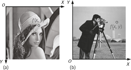
Equation (1.1) also provides a visual representation of a 2-D image as a spatial distribution pattern of certain properties (e. g., brightness). Each basic unit (corresponding to each entry in the matrix of eq. (1.1)) in 2-D image is called an image element (picture element in early days, so it is referred to as pixel). For a 3-D image in space XYZ, the basic unit is called voxel(comes from volume element). It can also be seen from eq. (1.1) that a 2-D image is a 2-D spatial distribution of a certain magnitude pattern. The basic idea of 2-D image display is often to regard a grayscale 2-D image as a luminance distribution at the 2-D spatial positions. Generally, a display device is used to display images at different spatial positions with different gray values, as in Example 1.1.
Figure 1.1 shows two typical grayscale images (Lena and Cameraman), which are displayed in two different forms, respectively. The coordinate system shown in Figure 1.1(a) is often used in the screen display. The origin O of the coordinate system is at the upper left corner of the image. The vertical axis marks the image row and the horizontal axis marks the image column. The coordinate system shown in Figure 1.1(b) is often used in image computation. Its origin O is at the lower left corner of the image, the horizontal axis is the X-axis, and the vertical axis is the Y-axis (the same as the Cartesian coordinate system). Note that f(x, y) can be used to represent this image and the pixel value at the pixel coordinates (x, y).
1.1.2Image Engineering
Image engineering is a new discipline, which combines the basic theory of mathematics, optics, and other basic principles with the accumulated experience in the development of the image applications. It collects the various image techniques to focus on the research and application of the entire image field.
Image technique, in a broad sense, is a general term for a variety of image-related technologies. In addition to the image acquisition and a variety of different operations on images, it can also include decision making and behavior planning based on the operating results, as well as the design, implementation, and production of hardware for the completion of these functions, as well as other related aspects.
1.1.2.1Three Levels of Image Engineering
Image engineering is very rich in content and has a wide coverage. It can be divided into three levels, namely image processing, image analysis, and image understanding, according to the degree of abstraction, data volume, and semantic level and operands, as shown in Figure 1.2. The first book in this set focused on image processing with relatively low level of operations. It treats mainly the image pixel with a very large volume of data. This book focuses on the image analysis that is in the middle level of image engineering, and both segmentation and feature extraction have converted the original pixel representation of the image into a relatively simple non-graphical description. The third book in this set focuses on image understanding, that is, mainly high-level operations. Basically it carries on the symbols representing the description of image. In this level, the process and method used can have many similarities with the human reasoning.

As shown in Figure 1.2, as the level of abstraction increases, the amount of data will be gradually reduced. Specifically, the original image data, through a series of processing, undergo steady transformation and become more representative and better organized useful information. In this process, on the one hand, the semantics get introduced, the operands are changed, and the amount of data is compressed. On the other hand, high-level operations have a directive effect on lower-level operations, thereby improving the performance of lower-level operations.
Example 1.2 From image representation to symbolic expression.
The original collected image is generally stored in the form of a raster image. The image area is divided into small cells, each of which uses a grayscale value between the maximum and minimum values to represent the brightness of the image at the cell. If the grating is small enough, that is, the cell size is small enough, a continuous image can be seen.
The purpose of image analysis is to extract data that adequately describe the characteristics of objects and use as little memory as possible. Figure 1.3 shows the change in expression that occurs in the raster image analyzed. Figure 1.3(a) is the original raster form of the image, and each small square corresponds to a pixel. Some pixels in the image have lower gray levels (shadows), indicating that they differ (in property) from other pixels around them. These pixels with lower grayscale form an approximately circular ring. Through image analysis, the circular object (a collection of some pixels in the image) can be segmented to get the contour curve as shown in Figure 1.3(b). Next, a (perfect) circle is used to fit the above curve, and the circle vector is quantized using geometric representation to obtain a closed smooth curve. After extracting the circle, the symbolic expression can be obtained. Figure 1.3(c) quantitatively and concisely gives the equation of the circle. Figure 1.3(d) abstractly gives the concept of “circle.” Figure 1.3(d) can be seen as a result or interpretation of the symbolic expression given by the mathematical formula in Figure 1.3(c). Compared to the quantitative expression (describing the exact size and shape of the object) of Figure 1.3(c), the interpretation in Figure 1.3(d) is more qualitative and more abstract.
Obviously, from image to object, from object to symbolic expression, and from symbolic expression to abstract concept, the amount of data are gradually reduced, and the semantic levels are gradually increased, along with the image processing, analysis, and understanding.![]()
1.1.2.2Papers Classification for Three Levels
The research and application of the three levels of image engineering are constantly developing. In the survey series of the image engineering that started since 1996, some statistical classifications for papers published are performed (Zhang, 2015e; 2017).
A summary of the number of publications concerning image engineering from 1995 to 2016 is shown in Table 1.1. In Table 1.1, the total number of papers published in these journals (#T), the number of papers selected for survey as they are related to image engineering (#S), and the selection ratio (SR) for each year, are provided.
Table 1.1: Summary of image engineering over 22 years.
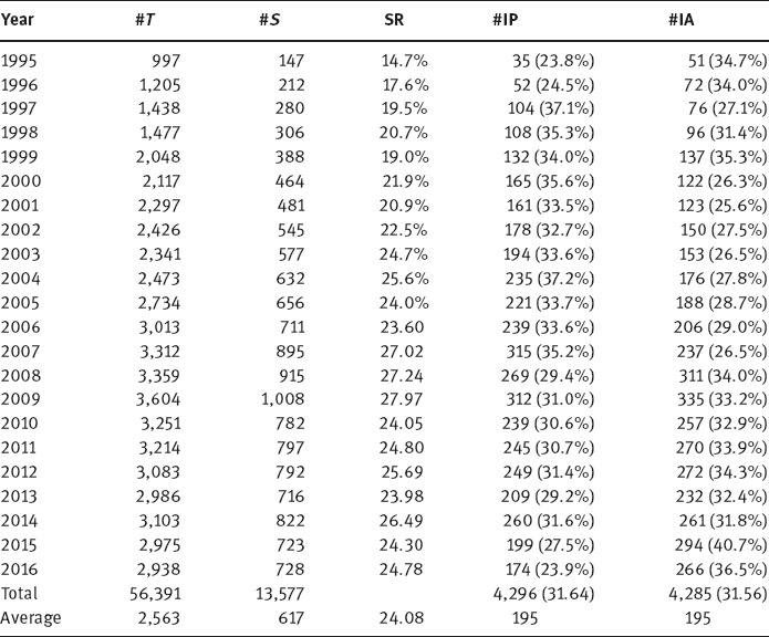

It is observed that image engineering is an (more and more) important topic for electronic engineering, computer science, automation, and information technology. The average SR is more than 1/5 (it is more than 1/4 in several recent years), which is remarkable in considering the wide coverage of these journals.
The selected papers on image engineering have been further classified into five categories: image processing (IP), image analysis (IA), image understanding (IU), technique applications (TA), and surveys.
In Table 1.1, the statistics for IP papers and IA papers are also provided for comparison. The listed numbers under #IP and #IA are the numbers of papers published each year belonging to image processing and to image analysis, respectively. The percentages in parenthesis are the ratios of #IP/#S and #IA/#S, respectively. The total number of papers related to image analysis is almost equal to the total number of papers related to image processing in these 21 years.
The proportions and variations of the number of papers in these years are shown in Figure 1.4. The papers related to image processing are generally the most in number, but the papers related to image analysis are on rise for many years steadily and occupies the top spot in recent years. At present, image analysis is considered the prime focus of image engineering.
1.2The Scope of Image Analysis
As shown in Figure 1.2, image analysis is positioned in the middle level of the image engineering. It plays an important role in connecting the upper level and lower level by using the results of image processing and by foundering image understanding.
1.2.1Definition and Research Content of Image Analysis
The definition of image analysis and its research contents are enclosed by the upper and lower layers of image engineering.
1.2.1.1Definition of Image Analysis
The definition and description of image analysis have different versions. Here are a few examples:
1.The purpose of image analysis is to construct a description of the scene based on the information extracted from the image (Rosenfeld, 1984).
2.Image analysis refers to the use of computers for processing images to find out what is in the image (Pavlidis, 1988).
3.Image analysis quantifies and classifies images and objects in images (Mahdavieh, 1992).
4.Image analysis considers how to extract meaningful measurement data from multidimensional signals (Young, 1993).
5.The central problem with image analysis is to reduce the grayscale or color images with a number of megabytes to only a few meaningful and useful digits (Russ, 2002).
In this book, image analysis is seen as the process and technique starting from an image, and detecting, extracting, representing, describing, and measuring the objects of interest inside, to obtain objective information and output data results.
1.2.1.2Differences and Connections Between Image Processing and Image Analysis
Image processing and image analysis have their own characteristics, which have been described separately in Section 1.1.2. Image processing and image analysis are also closely related. Many techniques for image processing are used in the process from collecting images to analyze the results. In other words, the work of image analysis is often performed on the basis of the results of image (pre)processing.
Image processing and image analysis are different. Some people think that image processing (such as word processing and food processing) is a science of reorganization (Russ, 2016). For a pixel, its attribute value may change according to the values of its neighboring pixels, or it can be itself moved to other places in the image, but the absolute number of pixels in the whole image does not change. For example, in word processing, the paragraphs can be cut or copied to perform phonics checks, or the fonts can be changed without reducing the amount of text. As in food processing, it is necessary to reorganize the ingredients to produce a better combination, rather than to extract the essence of various ingredients. However, the image analysis is different, and its goal is to try to extract the descriptive coefficients from the image (similar as the extraction of the essence of various ingredients in food processing), which can succinctly represent the important information in the image and can express quantitatively and effectively the content of the image.
Example 1.3 Process flow of image analysis.
Figure 1.5 shows a practical process flow and the main steps involved in a 3-D image analysis program:
1.Image acquisition: Obtaining the image from the original scene;
2.Preprocessing: Correcting the image distortion produced during the process of image acquisition;
3.Image restoration: Filtering the image after correction to reduce the influence of noise and other distortion;
4.Image segmentation: Decomposing the image into the target and other background for analyzing the image;
5.Object measurement: Estimating the “analog” property of the original scene from the digital image data;
6.Graphic generation: Providing the results of the measurement in a user-friendly and easy to understand way in a visualized display.
From the above steps the links between image processing and image analysis can be understood.![]()
1.2.1.3Image Analysis and Pattern Recognition
The main functional modules of image analysis are shown in Figure 1.6.
As shown in Figure 1.6, image analysis mainly includes the segmentation of the image, the representation/description of the object, as well as the measurement and analysis of the characteristic parameters of objects. In order to accomplish these tasks, many corresponding theories, tools, and techniques are needed. The work of image analysis is carried out around its operand—object. Image segmentation is to separate and extract the object from the image. The representation/description is to express and explain the object effectively, and the characteristic measurement and analysis are to obtain the properties of the object. Since the object is a set of pixels, image analysis places more emphasis on the relationships and connections between pixels (e. g., neighborhood and connectivity).

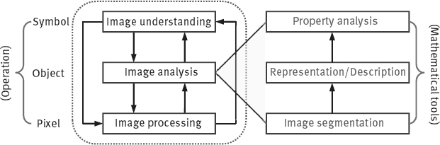
Image analysis and pattern recognition are closely related. The purpose of pattern recognition is to classify the different patterns. The separation of the objects from the background can be considered as a region classification. To further classify the regions, it is necessary to determine the parameters that describe the characteristics of the regions. A process flow of (image) pattern recognition is shown in Figure 1.7.
The input image is segmented to obtain the object image, the features of the object are detected, measured, and calculated, and the object can be classified according to the obtained feature measurements. In conclusion, image analysis and (image) pattern recognition have the same input, similar process steps or procedures, and convertible outputs.
1.2.1.4Subcategories of Image Analysis
From the survey series mentioned in Section 1.1.2, the selected papers on image engineering have been further classified into different categories such as image processing (IP) and image analysis (IA). The papers under the category IP have been further classified into five subcategories. Their contents and numbers of papers per year are listed in Table 1.2.

Table 1.2: The classification of image analysis category.
| Subcategory | #/Year |
| B1: Image segmentation, detection of edge, corner, interest points | 71 |
| B2: Representation, description, measurement of objects (bi-level image processing) | 12 |
| B3: Feature measurement of color, shape, texture, position, structure, motion, etc. | 17 |
| B4: Object (2-D) extraction, tracking, discrimination, classification, and recognition | 53 |
| B5: Human organ (biometrics) detection, location, identification, categorization, etc. | 53 |
1.2.2Image Analysis System
Image analysis systems can be constructed using a variety of image analysis devices and techniques and can be used to perform many image analysis tasks.
1.2.2.1History and Development
Image analysis has a long history. The following are some of the early events of the image analysis system (Joyce, 1985):
1.The first system to analyze images using a television camera was developed by a metal research institute. Its earliest model system was developed in 1963.
2.Electronic era really began in 1969, when a company in the United States (Bausch and Lomb) produced an image analyzer that could store a complete black-and-white image in a small computer for analysis.
3.In 1977, the company Joyce Loebl of the United Kingdom proposed a third-generation image analysis system, which uses software instead of hardware. The analysis function is separated from the image acquisition and becomes more general.
Image analysis systems have already obtained in-depth research, rapid development, and wide application, in the 1980s and 1990s of twentieth century. During this period, many typical system structures were proposed, and many practical application systems were established (Zhang, 1991a; Russ, 2016).
Image analysis system takes the hardware as the physical basis. A variety of image analysis tasks can generally be described in the form of algorithms, and most of the algorithms can be implemented in software, so there are many image analysis systems now only need to use a common general-purpose computer. Special hardware can be used in order to increase the speed of operation or to overcome the limitations of general-purpose computers. In the 1980s and 1990s of twentieth century, people have designed a variety of image cards compatible with industry-standard bus, which can be inserted into the computer or workstation. These image cards include image capture cards for image digitization and temporary storage, arithmetic and logic units for arithmetic and logic operations at video speeds, and memories such as frame buffers. Getting into the twenty-first century, the system’s integration is further improved, and system-on-chip (SOC) has also been rapidly developed. The progress of these hardware not only reduces the cost, but also promotes the development of special software for image processing and analysis. There are a number of image analysis systems and image analysis packages commercially available.
1.2.2.2Diagram of Analysis System
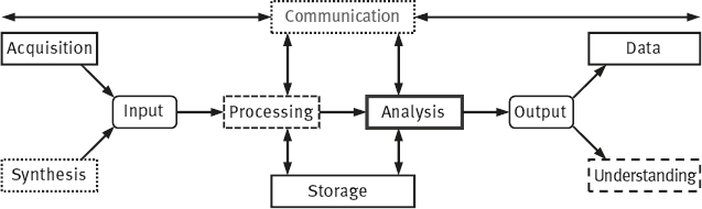
The structure of a basic image analysis system can be represented by Figure 1.8. It is similar to the framework of image-processing system, in which the analysis module is continued after the (optional) processing module. It has also specific modules for collecting, synthesizing, inputting, communicating, storing, and outputting functions. The final output of the analysis is either data (the data measured from the object in image and/or the resulting data of analysis) or the symbolic representation for further understanding, which is different from the image processing system.
Because that the basic information about processing modules has been covered in the first book of this set, the techniques of the analysis module will be discussed in detail in this (second) book. According to the survey on the literature of image engineering, the current image analysis researches are mainly concentrated in the following five aspects:
1.Edge detection, image segmentation;
2.Object representation, description, measurement;
3.Analysis of color, shape, texture, space, movement, and other characteristics of the objects;
4.Object detection, extraction, tracking, identification, and classification;
5.Human face and organ detection, positioning, and identification.
The following two sections give a brief introduction to some fundamental concepts and terminologies of the image analysis.
1.3Digitization in Image Analysis
The goal of image analysis is to obtain the measurement data of the interest objects in the image; these objects of interest are obtained by discretizing successive objects in the scene. Object is an important concept and the main operand in image analysis, which is composed of related pixels. Related pixels are closely linked both in the spatial locations and in the attribute characteristics. They generally constitute the connected components in image. To analyze the position link of the pixels, the spatial relationship among the pixels must be considered, where the discrete distance plays an important role. While to analyze the connectivity, not only the distance relationship but also the attribute relationship should be taken into account. In order to obtain accurate measurement data from the objects, an understanding of the digitization process and characteristics in analysis is required.
1.3.1Discrete Distance
In digital images, the pixels are discrete, the spatial relationship between them can be described by the discrete distance.
1.3.1.1Distance and Neighborhood
If assuming that p, q, and r are three pixels and their coordinates are (xp, yp), (xq, yq), and (xr, yr), respectively, then the distance functiond should satisfy the following three metric conditions:
1.d(p, q) ≥ 0 (d(p, q) = 0, if and only if p = q);
2.d(p, q) = d(q, p);
3.d(p, r) < d(p, q) + d(q, r).
The neighborhood of the pixels can be defined by distance. The four-neighborhood N4(p) of a pixel p(xp, yp) is defined as (see the pixel r(xr, yr) in Figure 1.9(a)):
N4(p)={r|d4(p,r)=1} (1.2)
The city block distanced4(p, r) = |xp – xr| + |yp – yr|.
The eight-neighborhood N8(p) of a pixel p(xp, yp) is defined as the AND set of its four-neighborhood N4(p) and its diagonal neighborhood ND(p) (see pixels marked by s in Figure 1.9(b)), that is:
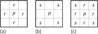
N8(p)=N4(p)∪ND(p) (1.3)
So the eight-neighborhood N8(p) of a pixel p(xp, yp) can also be defined as (see the pixels marked by r and s in Figure 1.9(c)):
N8(p)={r|d8(p,r)=1} (1.4)
The chessboard distanced8(p, r) = max(|xp – xr|, |yp – yr|).
1.3.1.2Discrete Distance Disc
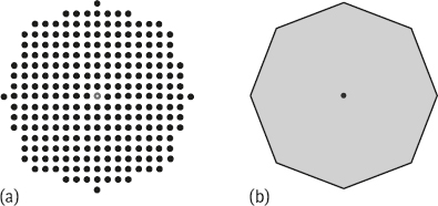
Given a discrete distance metric dD, a disc with radius R (R ≥ 0) and centered on pixel p is a point set satisfying ∆D(p, R) = {q|dD(p, q) ≤ R}. When the position of the center pixel p can be disregarded, the disc with radius R can also be simply denoted by ∆D(R).
Let ∆i(R), i = 4,8, represent an equidistant disc with the distance di from the center pixel less than or equal to R, and #[∆i(R)] represent the number of pixels, except center pixel, in ∆i(R), then the number of pixels increases in proportion with distance. For the city block disc, there is
#[Δ4(R)]=4R∑j=1j=4(1+2+3+⋯+R)=2R(R+1) (1.5)
Similarly, for the chessboard disc, there is
#[Δ8(R)]=8R∑j=1j=8(1+2+3+⋯+R)=4R(R+1) (1.6)
In addition, the chessboard disc is actually a square, and so the following formula can also be used to calculate the number of pixels, except the central pixel, in the chessboard disc
#[Δ8(R)]=(2R+1)2−1 (1.7)
Here are a few different values of ∆i(R): #[∆4(5)] = 60, #[∆4(6)] = 84, #[∆8(3)] = 48, #[∆8(4)] = 80.
1.3.1.3The Chamfer Distance
The chamfer distance is an integer approximation to the Euclidean distance in the neighborhood. Traveling from pixel p to its 4-neighbors needs simply a horizontal or vertical move (called a-move). Since all displacements are equal according to the symmetry or rotation, the only possible definition of the discrete distance is d4 distance, where a = 1. Traveling from pixel p to its 8-neighborhood cannot be achieved by only a horizontally or vertically move, a diagonal move (called b-move) is also required. Combining these two moves, the chamfer distance is obtained, and can be recorded as da,b. The most natural value for b is 21/2a, but for the simplicity of calculation and for reducing the amount of memory, both a and b should be integers. The most common set of values is a = 3 and b = 4. This set of values can be obtained as follows. Considering that the number of pixels in the horizontal direction between two pixels p and q is nx and the number of pixels in vertical direction between two pixels p and q is ny (without loss of generality, let nx > ny), then the chamfer distance between pixels p and q is
D(p,q)=(nx−ny)a+nyb (1.8)
The difference between the chamfer distance and Euclidean distance is
ΔD(p,q)=√n2x+n2y−[(nx−ny)a+nyb] (1.9)
If a = 1, b = √2
ΔD′(p,q)=ny√n2x+n2y−(√2−1) (1.10)
Let the above derivative be zero, computing the extreme of ∆D(p, q) gives
ny=√(√2−1)/2nx (1.11)
The difference between the two distances, ∆D(p, q), will take the maximum value (23/2 – 2)1/2nx ≈ –0.09nx when meeting the above equation (the angle between the straight line and the horizontal axis is about 24.5°). It can be further proved that the maximum of ∆D(p, q) can be minimized when b = 1/21/2 + (21/2 – 1)1/2 = 1.351. As 4/3 ≈ 1.33, so in the chamfer distance a = 3 and b = 4 are taken.
Figure 1.10 shows two examples of equidistant discs based on the chamfer distance, where the left disc is for ∆3,4(27), and the right disc is for ∆a,b.
1.3.2Connected Component
The object in image is a connected component composed of pixels. A connected component is a set of connected pixels. Connection needs to be defined according to the connectivity. A connectivity is a relationship between two pixels, in which both their positional relation and their magnitude relation are considered. Two pixels having connectivity are spatially adjacent (i. e., one pixel is in the neighborhood of another pixel) and are similar in magnitude under certain criteria (for grayscale images, their gray values should be equal, or more generally in a same grayscale value set V).
It can be seen that the adjacency of two pixels is one of the necessary conditions for these two pixels to be connected (the other condition is that they are taken values from a same grayscale value set V). As shown in Figure 1.10, two pixels may be 4-adjacent (one pixel is within a 4-neighborhood of another pixel), or 8-contiguous (one pixel is within an 8-neighborhood of another pixel). Correspondingly, two pixels maybe 4-connected (these two pixels are 4-adjacent), or 8-connected (these two pixels are 8-adjacent).
In fact, it is also possible to define another kind of connection, m-connection (mixed connection). If two pixels, p and r, take values in V and satisfy one of the following conditions, then they are m-connected: (1) r is in N4(p); (2) r is in ND(p) and there is no pixel with value in V included in N4(p) ∩ N4(r). For a further explanation of the condition (2) in the mixed connection, see Figure 1.11. In Figure 1.11(a), the pixel r is in ND(p), N4(p) consists of four pixels denoted by a, b, c, d, N4(r) consists of four pixels denoted by c, d, e, f, and N4(p) ∩ N4(r) includes two pixels labeled c and d. Let V = {1}, then Figure 1.11(b, c) gives an example of satisfying and no-satisfying condition (2), respectively. In the two figures, the two shaded pixels are each other in the opposite diagonal neighborhoods, respectively. However, the two pixels in Figure 1.11(b) do not have a common neighbor pixel with value 1, while the two pixels in Figure 1.11(c) do have a common neighbor pixel with value 1. Thus, the pixels p and r are m-connected in Figure 1.11(b) and the m-connection between the pixels p and r in Figure 1.11(c) does not hold (they are connected via pixel c).
As discussed earlier, the mixed connection is essentially to take a 4-connection when both 4-connection and 8-connection are possible for two pixels, and to shield the 8-connection between the two pixels having 4-connections with a same pixel. A mixed connection can be thought of as a variant of the 8-connection, whose introduction is to eliminate the multiplexing problem that often occurs with 8-connections. Figure 1.12 shows an example. In Figure 1.12(a), the pixel labeled 1 forms the boundary of a region consisting of three pixels with values 0. When this boundary is considered as a path, there are two paths between the three pixels at each of the four corners, which is the ambiguity caused by the use of an 8-connection. This ambiguity can be eliminated by using m-connection, and the results are shown in Figure 1.12(b). Since the direct m-connection between the two diagonal pixels cannot be established (the two conditions for the mixed connection are not satisfied), there is now only one path, which has no ambiguous problem.


Connection can be seen as an extension of connectivity. It is a relationship created by two pixels with the help of other pixels. Consider a series of pixels {pi(xi, yi), i = 0, n}. When all pi(xi, yi) are connected with pi–1(xi–1, yi–1), then two pixels p0(x0, y0) and pn(xn, yn) are connected through other pixels pi(xi, yi). If pi(xi, yi) has 4-connectivity with pi–1(xi–1, yi–1), then p0(x0, y0)and pn(xn, yn) are 4-connected. If pi(xi, yi) has 8-connectivity with pi–1(xi–1, yi–1), then p0(x0, y0) and pn(xn, yn) are 8-connected. If pi(xi, yi) has m-connectivity with pi–1(xi–1, yi–1), then p0(x0, y0) and pn(xn, yn) are m-connected.
A series of pixels connected as above constitutes a connected component in the image, or an image subset, or a region. In a connected component, any two pixels are connected by the connectivity of other pixels in the component. For two connected components, if one or several pixels in a connected component are adjacent to one or several pixels in another connected component, these two connected components are adjacent; if one or several pixels in a connected component have connectivity with one or several pixels in another connected component, these two connected components are connected, and these two connected components can form one connected component.
1.3.3Digitizing Model
The digitizing model discussed here is used to transform spatially continuous scenes into discrete digital images, so it is a spatial quantization model.
1.3.3.1Fundamentals
Here are some basic knowledge of the digitizing model (Marchand 2000)

The preimages and domain of the digitized set P are first defined:
1.Preimage: Given a set of discrete points P, a set of consecutive points S that is digitized as P is called a preimage of P;
2.Domain: The region defined by the union of all possible preimages S is called the domain of P.
There are a variety of digitizing models, in which the quantization is always a many-to-one mapping, so they are irreversible processes. Thus, the same quantized result image may be mapped from different preimages. It can also be said that the objects of different sizes or shapes may have the same discretization results.
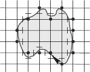
Now consider first a simple digitizing model. A square image grid is overlaid on a continuous object S, and a pixel is represented by an intersection point p on the square grid, which is a digitized result of S if and only if p ∈ S. Figure 1.13 shows an example where S is represented by a shaded portion, a black dot represents a pixel p belonging to S, and all p make up a set P.
Here, the distance between the image grid points is also known as the sampling step, which can be denoted h. In the case of a square grid, the sampling step is defined by a real value, and h > 0, which defines the distance between two 4-neighbor pixels.
Example 1.4 Effect of different sampling steps.
In Figure 1.14(a), the continuous set S is digitized with a given sampling step h. Figure 1.14(b) gives the result for the same set S being digitized with another sampling step h′ = 2h. Obviously, such an effect is also equivalent to changing the size of successive sets S by the scale h/h′ and digitizing with the original sampling step h, as shown in Figure 1.14(c).![]()
An analysis of this digitizing model shows that it may lead to some inconsistencies, as illustrated in Figure 1.15:
1.A nonempty set S may be mapped to an empty digitizing set. Figure 1.15(a) gives several examples in which each nonempty set (including two thin objects) does not contain any integer points.
2.This digitizing model is not translation invariant. Figure 1.15(b) gives several examples where the same set S may be mapped to an empty, disconnected, or connected digitized set (the numbers of points in each set are 0, 2, 3, 6, respectively) depending on its position in the grid. In the terminology of image processing, the change of P with the translation of S is called aliasing.

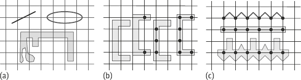
3.Given a digitized set P, it is not guaranteed to accurately characterize its preimage S. Figure 1.15(c) shows a few examples where three dissimilar objects with very different shapes provide the same digitized results (points in a row).
As discussed earlier, a suitable digitizing model should have the following characteristics:
1.The digitized result for a nonempty continuous set should be nonempty.
2.The digitizing model should be as translation-invariant as possible (i.e., the aliasing effect should be as small as possible).
3.Given a set P, each of its preimages should be similar under certain criteria. Strictly speaking, the domain of P should be limited and as small as possible.
Commonly used digitizing models are square box quantization (SBQ), grid-intersect quantization (GIQ) and object contour quantization (Zhang, 2005b). Only the SBQ and GIQ digitizing models are introduced below.
1.3.3.2The Square Box Quantization
In SBQ, there is a corresponding digitization box Bi = (xi – 1/2, xi + 1/2) × (yi – 1/2, yi + 1/2) for any pixel pi = (xi, yi). Here, a half-open box is defined to ensure that all boxes completely cover the plane. A pixel pi is in the digitized set P of preimage S if and only if Bi ∩ S ≠ ∅, that is, its corresponding digitizing cell Bt intersects S. Figure 1.16 shows the set of digitization (square box with a dot in center) obtained by SBQ from the continuous point set S in Figure 1.13. Wherein the dotted line represents a square segmentation, which is dual with the quadratic sampling grid. It can be seen from the figure that if the square corresponding to a pixel intersects S, then this pixel will appear in the digitizing set produced by its SBQ. That is, the digitized set P obtained from a continuous point set S is the pixel set {pi|Bi ∩ S ≠ ∅}.


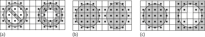
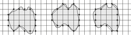
The result of SBQ for a continuous line segment is a 4-digit arc. The definition of SBQ guarantees that a nonempty set S will be mapped to a nonempty discrete set P, since each real point can be guaranteed to be uniquely mapped to a discrete point. However, this does not guarantee a complete translation invariance. It can only reduce greatly the aliasing. Figure 1.17 shows several examples in which the continuous sets are the same as in Figure 1.15(b). The numbers of points in each discrete set are 9, 6,9, 6, respectively, which are closer each other than that in Figure 1.15(b).
Finally, it should be pointed out that the following issues in SBQ have not been resolved (Marchand, 2000):
1.The number of connected components in the background may not be maintained. In particular, the holes in S may not appear in P, as shown in Figure 1.18(a), where the dark shaded area represents S (with two holes in the middle), and the black point set represents P (no holes in the middle).
2.Since S ⊂ ∪iBi, the number NS of connected components in a continuous set S is not always equal to the number NP of connected components in its corresponding discrete set P, generally NS ≤ NP. Figure 1.18(b) shows two examples where the number of black points in the dark-shaded area representing S is less than the number of black dots in the shallow shaded area representing P.
3.More generally, the discrete set P of a continuous set S has no relation to the discrete set Pc of a continuous set Sc, where the superscripts denote the complement. Figure 1.18(c) shows two examples in which the dark-shaded area on the left represents S and the black-point set represents P; the dark-shaded area on the right represents Sc, and the black-point set represents Pc. Comparing these two figures, it is hardly to see the complementary relationship between P and Pc.
1.3.3.3Grid-Intersect Quantization
GIQ can be defined as follows. Given a thin object C formed by continuous points, its intersection with the grid line is a real point t = (xt, yt). This point may satisfy xt ∈ I or yt ∈ I (where I represents a set of 1-D integers) depending on that C intersects the vertical grid lines or the horizontal grid lines. This point t ∈ C will be mapped to a grid point pi = (xi, yi), where t ∈ (xi – 1/2, xi + 1/2) × (yi – 1/2, yi + 1/2). In special cases (such as xt = xi + 1/2 or yt = yi + 1/2), the point pi located at left or top will be taken as belonging to the discrete set P.
Figure 1.19 shows the results obtained for a curve C using the GIQ. In this example, C is clockwise (as indicated by the arrow in the figure) traced. Any short continuous line between C and the pixel marked by dot is mapped to the corresponding pixel.
It can be proved that the result of GIQ for a continuous straight line segment (α, β) is an 8-digit arc. Further, it can be defined by the intersection of (α, β) and the horizontal or vertical (depending on the slope of (α, β) line.
GIQ is often used as a theoretical model for image acquisition. The aliasing effects generated by the GIQ are shown in Figure 1.20. If the sampling step h is appropriate for the digitization of C, the resulting aliasing effect is similar to the aliasing effect produced by SBQ.

A comparison of the GIQ domain and the SBQ domain is given in the following. Figure 1.21(a) gives the result of digitizing the curve C by the SBQ method (all black dots). Pixels surrounded by small squares are those that do not appear in the GIQ result of digitizing the curve C. Clearly, GIQ reduces the number of pixels in a digitized set. On the other hand, Figure 1.21(b) shows the domain boundaries derived from the GIQ and SBQ results for corresponding C. The dotted line represents the boundary of the union of successive subsets defined by the GIQ result, and the thin line represents the boundary of the union of successive subsets defined by the SBQ result.
As shown in Figure 1.21, the area of the SBQ domain is smaller than the area of the GIQ domain. In this sense, SBQ is more accurate in characterizing a preimage of a given digitized set. However, the shape of the GIQ domain appears to be more appropriate for the description of the curve C than the shape of the SBQ domain. The explanation is that if the sampling step is chosen so that the details in Care larger than the size of the square grid, these details will intersect with the different grid lines. Further, each such intersection will be mapped to one pixel, and such pixels determine a contiguous subset as shown in Figure 1.21(a). In contrast, SBQ maps these details to a group of 4-adjacent pixels that define a wider contiguous region, which is the union of the corresponding digital boxes.
1.3.4Digital Arcs and Chords
In Euclidean geometry, the arc is a part of the curve between two points, while the chord is the straight line connecting any two points on the conic curve. A continuous straight line segment can often be viewed as a special case of an arc.
A digitized set is a discrete set obtained by digitizing a continuous set using a digitizing model. In the study of discrete objects, they can be seen as a digitization results of continuous objects. The property of a continuous object that has been demonstrated in Euclidean geometry can be mapped to a discrete set. The digital arcs and digital chords, as well as some of their properties, are discussed below.
1.3.4.1Digital Arcs
Given a neighborhood and the corresponding movement length, the chamfer distance between two pixels p and q with respect to this neighborhood is the length of the shortest digital arc from p to q. Here, the digital arc may be defined as follows. Given a set of discrete points and the adjacency between them, the digital arc Ppq from point p to point q is defined as the arc Ppq = {pi, i = 0, 1,..., n} satisfying the following conditions (Marchand, 2000):
1.p0=p,pn=q;
2.∀i = 1, …, n–1, point p has exactly two adjacent points in the arc Ppq:pi–1 and pi+1;
3.The endpoint p0(or pn) has exactly one adjacent point in the arc Ppq: p1 (or pn–1).
Different digital arcs (4-digit arcs or 8-digit arcs) can be defined as above, depending on the difference in adjacency (e. g., 4-adjacent or 8-adjacent).
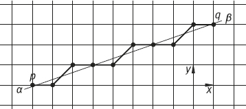
Consider the continuous straight line segment [α, β] (the segment from α to β) in the square grid given in Figure 1.22. Using GIQ, points intersecting the grid lines between [α, β] are mapped to their nearest integer points. When there are two equal-distance closest points, the left discrete point in [α, β] can be first selected. The resulting set of discrete points {pi}i=0,...,n is called a digitized set of [α, β].
1.3.4.2Digital Chords
Discrete linearity is first discussed below, then whether a digital arc is a digital chord will be discussed.
The determination of the digital chord is based on the following principle: Given a digital arc Ppq = {pi}i=0,..., n from p = p0 to q = pn, the distance between the continuous line [pi, pj] and the sum of the segments ∪j[pj, pi+1] can be measured using the discrete distance function and should not exceed a certain threshold (Marchand, 2000). Figure 1.23 shows two examples where the shaded area represents the distance between Ppq and the continuous line segments [pi, pj].
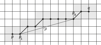
It can be proved that given any two discrete points pi and pj in an 8-digit arc Ppq = {pi}i = 0,..., n and the real point1 in any continuous line segment [pi, pj], if there exists a point pk ∈ Ppq such that d8(ρ, pk) < 1, then Ppq satisfies the property of the chord.
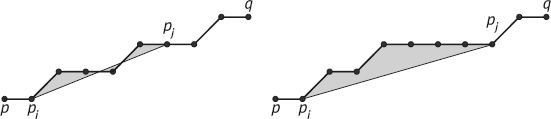
To determine the property of the chord, a polygon that surrounds a digital arc can be first defined, which can include all the continuous segments between the discrete points on the digital arc (as shown by the shaded polygons in Figures 1.24 and 1.25). This polygon will be called a visible polygon, since any other point can be seen from any point in the polygon (i.e., the two points can be connected by a straight line in the polygon). Figures 1.24 and 1.25 show two examples of verifying that the chord properties are true and not true, respectively.
In Figure 1.24, there is always a point pk ∈ Ppq such that d8(ρ, pk) < 1 for all points in the shadow polygon of the digital arc Ppq. In Figure 1.25, there is ρ ∈ (p1, p8) that can have d8(ρ, pk) ≥ 1 for any k = 0, ..., n. In other words, ρ is located outside the visible polygon, or p8 is not visible from p1 in the visible polygon (and vice versa). The failure of chord property indicates that Ppq is not the result of digitizing a line segment.
It can be proved that in the 8-digital space, the result of the line digitization is a digital arc that satisfies the properties of the chord. Conversely, if a digital arc satisfies the property of the chord, it is the result of digitizing the line segments (Marchand, 2000).
1.4Distance Transforms
DT is a special transform that maps a binary image into a grayscale image. DT is a global operation, but it can be obtained by local distance computation. The main concepts involved in DT are still neighborhood, adjacency, and connectivity.

1.4.1Definition and Property
DT computes the distance between a point inside a region and the closest point outside the region. In other words, the DT of a point in a region computes the nearest distance between this point and the boundary of the region. Strictly speaking, DT can be defined as follows: Given a set of points P, a subset B ∈ P, and a distance function D(.,.) that satisfies the metric conditions in Section 1.3.1, the distance transformation DT(.) of a point p ∈ P is
DT(p)=minq∈B{D(p,q)} (1.12)
The ideal measurement for distance is Euclidean distance. However, for the sake of simplicity, distance functions with integer-based arithmetic are often used, such as D4(.,.) and D8(.,.).
DT can generate a distance map of P, which is represented by a matrix [DT(p)]. The distance map has the same size as the original image and stores the value of DT(p) for each point p ∈ P.
Given a set of points P and one of its subsets B, the distance transformation of P satisfies the following properties:
1.DT(p) = 0 if and only if p ∈ B.
2.Defining the point ref(p) ∈ B such that DT(p) is defined by D[p, ref(p)] (ref(p) is the closest point to p in B) and the set of points {p|ref(p) = q} forms the Voronoi cell of point q. If ref(p) is nonunique, p is on the border of the Voronoi cell.
Given a set P and its border B, the distance transformation of P has the following properties (Marchand, 2000):
1.According to the definition of DT(.), DT(p) is the radius of the largest disc within P that is centered at p.
2.If there is exactly one point q ∈ B such that DT(p) = d(p, q), then there exists a point r ∈ P such that the disc of radius DT(r) centered at r contains the disc of radius DT(p) centered at p.
3.Conversely, if there are at least two points q and q′ in B such that DT(p) = d(p, q) = d(p, q′), then there is no disc within P that contains the disc of radius DT(p) centered at p. In that case, p is said to be the center of the maximal disc.
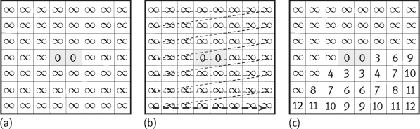
Example 1.5 Illustration of discrete distance map.
A distance map can be represented by a gray-level image, in which the value of each pixel is proportional to the value of the DT. Figure 1.26(a) is a binary image. If the edge of the image is regarded as the contour of the object region, Figure 1.26(b) is its corresponding gray-level image. The central pixels have higher gray-level values than the pixels near the boundary of the region. If the two white pixels in the center are regarded as a subset B, Figure 1.26(c) is its corresponding gray-level image. The center values are the smallest and the pixels surround have values increasing with the distance from the center.![]()

1.4.2Computation of Local Distances
Computing the distance using eq. (1.12) requires many calculations as it is a global operation. To solve this problem, an algorithm using only the information of the local neighborhood should be considered.
Given a set of discrete points P and one of its subsets B, Dd is the discrete distance used to compute the distance map of P. Then, for any point p ∈ P – B, there exists a point q, which is a neighbor of p (i. e., q ∈ ND(p)), such that DTD(p), the discrete distance transformation value at p, satisfies DTD(p) = DTD(q) + dD(p, q). Moreover, since p and q are neighbors, l(p, q) = dD(p, q) is the length of the move between p and q. Therefore, for any point p ∉ B, q can be described by DTD(q′) = min {DTD(p) + l(p, q′); q′ ∈ ND(p)}.
Both sequential and parallel approaches take advantage of the above property to efficiently compute discrete distance maps. A mask is defined which contains the information of local distances within the neighborhood p ∈ P. This mask is then centered at each point p ∈ P and the local distances are propagated by summing the central value with the corresponding coefficients in the mask.
A mask M(k, l) of size n × n for computing DT can be represented by an n × n matrix M(k, l), in which each element represents the local distance between pixelp = (xp, yp) and its neighbor q = (xp + k, yp + l). Normally, the mask is centered at pixel p, and n should be an odd value.
Figure 1.27 shows several examples of such masks for the propagation of local distances p. The shaded area represents the center of the mask (k = 0, l = 0). The size of the mask is determined by the type of the neighborhood considered. The value of each pixel in the neighborhood of p is the length of the respective move from p. The value of the center pixel is 0. In practice, the infinity sign is replaced by a large number.
The mask of Figure 1.27(a) is based on 4-neighbors and is used to propagate D4 distance. The mask of Figure 1.27(b) is based on 8-neighbors and is used to propagate D8 distance or Da,b (a = 1, b = 1) distance. The mask of Figure 1.27(c) is based on 16 neighbors and is used to propagate Da,b,c distance.

The process of calculating discrete distance maps using masks can be summarized as follows. Consider a binary image of size W×H and assume the set of its border point set B is known. The discrete distance map is a matrix, which is denoted [DT(p)], of size W×H and is calculated by iteratively updating its values until a stable state is reached. The distance map is initialized as (iteration t = 0)
DT(0)D(p)={0 if p∈B∞ if p∈B (1.13)
Then, for iterations t > 0, the mask M(k, l) is positioned at a pixel p = (xp, yp) and the following updating formula is used to propagate the distance values from the pixel q = (xp + k, yp + l) onto p
DT(t)D(p)=mink,l{DT(t−1)D(q)+M(k,l); q=(xp+k,yp+l)} (1.14)
The updating process stops when no change occurs in the distance map for the current iteration.
1.4.3Implementation of Discrete Distance Transformation
There are two types of techniques that can be used for the implementation of discrete distance transformation: sequential implementation, and parallel implementation. Both produce the same distance map (Borgefors, 1986).
1.4.3.1Sequential Implementation
For sequential implementation, the mask is divided into two symmetric submasks. Then, each of those submasks is sequentially applied to the initial distance map containing the values as defined by eq. (1.13) in a forward and backward raster scan, respectively.

Example 1.6 Sequential computation of a discrete distance map.
Consider the image shown in Figure 1.28(a) and the 3 × 3 mask (with a = 3 and b = 4) in Figure 1.28(b). The set B is defined as the central white pixels and P is the set of all pixels. The mask is first divided into two symmetric submasks, as shown in Figure 1.28(c, d), respectively.![]()
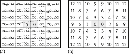
Forward pass: The initial distance map [DTD(p)](0) is shown in Figure 1.29(a). The upper submask is positioned at each point of the initial distance map and the value of each pixel is updated by using eq. (1.14), according to the scanning order shown in Figure 1.29(b). For values corresponding to the border of the image, only coefficients of the mask that are contained in the distance map are considered. This pass results in the distance map [DTD(p)](t′) shown in Figure 1.29(c).
Backward pass: In a similar way, the lower submask is positioned at each point of the distance map [DT(p)](t′) and the value of each pixel is updated by using eq. (1.14), according to the scanning order shown in Figure 1.30(a). This pass results in the distance map of the image shown in Figure 1.30(b).
Clearly, the complexity of this algorithm is O(W × H) since the updating formula in eq. (1.14) can be applied in constant time.
1.4.3.2Parallel Implementation
In parallel implementation, each pixel is associated with a processor. The discrete distance map is first initialized using eq. (1.13), and the updating operation given by eq. (1.14) is applied to all pixels for each iteration. The process stops when no change occurs in the discrete distance map for the current iteration.
The parallel implementation can be represented by (p = (xp, yp))
DT(t)(xp,yp)=mink,j{DT(t−1)(xp+k,yp+l)+M(k,l)} (1.15)
where DT(t)(xp, yp) is the iterative value at (xp, yp) for the tth iteration, k and l are the relative positions with respect to the center of mask (0, 0), and M(k, l) represents the mask entry value.
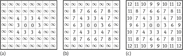
Example 1.7 Parallel computation of a discrete distance map.
Consider again the image shown in Figure 1.26(a). The mask used here is still the original distance mask shown in Figure 1.28(b) and the initial discrete distance map is shown in Figure 1.29(a). Figure 1.31(a, b) gives the first two temporary discrete distance maps obtained during the parallel computation. The distance map in Figure 1.31(c) is the final result.![]()
1.5Overview of the Book
This book has eight chapters. This chapter provides an overview of image analysis. The scope of image analysis is introduced along with a discussion on related topics. Some discrete distance metrics, digitization models, and the DT techniques that are specifically important for achieving the goal of image analysis (obtain the measurement data of the interest objects in image) are introduced.
Chapter 2 is titled image segmentation. This chapter introduces first the definition of segmentation and the classification of algorithms. Then, the four groups of basic techniques, as well as the extensions and generations of basic techniques are detailed. Finally, the segmentation evaluation is also discussed.
Chapter 3 is titled object representation and description. This chapter introduces first the schemes for representation classification and description classification. Then, the boundary-based representation, region-based representation, transform-based representation, the descriptors for boundary, and the descriptors for region are presented in sequence.
Chapter 4 is titled feature measurement and error analysis. This chapter discusses about direct and indirect measurements, the accuracy and precision of measurements, and the two commonly used types of connectivity. The sources of feature measurement errors are analyzed in detail. One example of error analysis procedure is also introduced.
Chapter 5 is titled texture analysis. This chapter introduces the concepts of texture and the classification of analysis approaches. The topics as statistical approaches, structural approaches, spectral approaches, texture categorization techniques, and texture segmentation techniques are discussed.
Chapter 6 is titled shape analysis. This chapter presents the definitions of shape and the tasks in shape analysis, and the different classes of 2-D shape. The main emphases are on the shape property description, technique-based descriptors, wavelet boundary descriptors, and the principle of fractal geometry for shape measurements.
Chapter 7 is titled motion analysis. This chapter provides an introduction to objective and tasks of motion analysis. The topics as motion detection, moving object detection, moving object segmentation, and moving object tracking are discussed with respective examples in details.
Chapter 8 is titled mathematical morphology. This chapter introduces both binary mathematical morphology and grayscale mathematical morphology. All are starting from basic operations, then further going to combined operations, and finally arriving at some practical algorithms.
Each chapter of this book is self-contained and has similar structure. After a general outline and an indication of the contents of each section in the chapter, the main subjects are introduced in several sections. Toward the end of every chapter, 12 exercises are provided in the Section “Problems and Questions.” Some of them involve conceptual understanding, some of them require formula derivation, some of them need calculation, and some of them demand practical programming. The answers or hints for two of them are collected and presented at the end of the book to help readers to start.
The references cited in the book are listed at the end of the book. These references can be broadly divided into two categories. One category relates directly to the contents of the material described in this book, the reader can find the source of relevant definitions, formula derivations, and example explanation. References of this category are generally marked at the corresponding positions in the text. The other category helps the reader for further study, for expanding the horizons or solving specific problems in scientific research. References of this category are listed in the Section “Further Reading” at the end of each chapter, where the main contents of these references are simply pointed out to help the reader targeted to access.
To read this book, some basic knowledge is essential:
1.Mathematics: Both Linear algebra and matrix theory are important, as the image is represented by a matrix, and image processing often requires matrix manipulation. In addition, knowledge of statistics, probability theory, and stochastic modeling is also very worthwhile.
2.Computer science: Mastery of computer software technology, understanding of the computer architecture system, and application of computer programming methods are very important.
3.Electronics: Many devices involved in image processing are electronic devices, such as camera, video camera, and display screen. In addition, electronic board, FPGA, GPU, SOC, and so on are frequently used.
Some specific prerequisites for reading this book include understanding the fundamentals of signal processing and some basic knowledge of image processing (Volume I, see also Zhang 2012b).
1.6Problems and Questions
![]()
1-1The video sequence includes a set of 2-D images. How can the video sequence be represented in matrix form? Are there other methods of representation?
1-2What are the relationships and differences between image analysis and image processing as well as image analysis and image understanding?
1-3*Using the database on the Internet, make a statistical investigation on the trends and characteristics of the development of image analysis in recent years.
1-4Looking up the literature to see what new mathematical tools have been used in image analysis in recent years? What results have been achieved?
1-5Looking up the literature to see what outstanding progress has been made in image acquisition and image display related to image analysis in recent years? What effects do they have on image analysis?
1-6What are the functional modules included in the image analysis system? What is the relationship among each other? Which modules have been selected by this book for presentation? What relationships have they with the modules of the image processing system?
1-7*Draw the chamfer discs of ∆3,4(15) and ∆3,4(28), respectively.
1-8For the digitized set obtained in Figure 1.16, the outermost pixels can be connected to form a closed contour according to the 4-connection and the 8-connection, respectively. It is required to determine whether or not they are digital arcs.
1-9Design a nonempty set S, which may be mapped to an empty digitized set in both two digitization models. Make a schematic diagram.
1-10With reference to Figure 1.18, discuss what would be the results if using grid-intersect quantization?
1-11Perform the distance transformation for the images in Figure Problem 1-11 using the serial algorithm and plot the results after each step.

1-12Computer the distance transform map for the simple shape in Figure Problem 1-12. Explain the meaning of the values in the resulted map.

1.7Further Reading
![]()
–More detailed introductions on image can be found in Volume I (Zhang, 2012b).
–The series of survey papers for image engineering can be found in Zhang (1996a, 1996b, 1997a, 1998a, 1999a, 2000a, 2001a, 2002a, 2003a, 2004, 2005a, 2006a, 2007a, 2008a, 2009, 2010, 2011a, 2012a, 2013a, 2014, 2015a, 2016 and 2017). Some summaries on this survey series can be found in Zhang (11996d, 2002c, 2008b and 2015e).
2.The Scope of Image Analysis
–More comprehensive introduction and further discussions on image analysis can be found in Joyce (1985), Lohmann (1998), Zhang (1999b), Kropatsch (2001), Umbaugh (2005), Zhang (2005b), Pratt (2007), Gonzalez (2008), Sonka (2008), Zhang (2012c) and Russ (2016).
3.Digitization in Image Analysis
–Extensions to neighborhood and discrete distance, including 16 neighborhood and distance can be found in Zhang (2005b).
–The introduction to the connectivity and the shortest path of the N16 space can be seen in Zhang (1999b).
4.Distance Transforms
–The method of 3-D distance transformation can be seen in Ragnemalm (1993).
5.Overview of the Book
–The main materials in this book are extracted from the books: Zhang (2005b), Zhang (2012c).
–More solutions for some problems and questions can be found in Zhang (2002b).
–More related materials can be found in Zhang (2007b) and Zhang (2013b).
–Particular information on the analysis of face images can be found in Lin (2003), Tan (2006), Yan (2009), Li (2011a), Tan (2011), Yan (2010), Zhu (2011), Zhang (2015b).