
6Shape Analysis
Shapes play an important role in describing the objects in images. Shape analysis is an essential branch of image analysis. The analysis of a shape should be based on shape properties and various available techniques. On the one hand, a property can be described by several techniques/descriptors. On the other hand, a technique can describe several properties of a shape.
The sections of this chapter are arranged as follows:
Section 6.1 overviews first the description and definition of shape and then summarizes the main research works for shape.
Section 6.2 describes a classification scheme for the shape of a plane object. The concept and property of each class are further explained to provide an overall understanding of the shape description.
Section 6.3 focuses on the description of the same shape features with different theoretical techniques. In particular, the methods for describing the compactness of shape with the ratio of appearance ratio, shape factor, spherical shape, circularity and eccentricity, and the methods for describing the shape complexity with simple descriptors, saturation and histogram of fuzzy graphs are presented.
Section 6.4 discusses the methods of describing different shape characteristics based on the same technique. The approaches with shape number comparison and region marker based on polygon representation, and the descriptor based on curvature calculation are introduced.
Section 6.5 focuses on the wavelet boundary descriptors that are formed by the coefficients of the wavelet transform of the object boundary. Its properties are provided and compared with Fourier boundary descriptors.
Section 6.6 describes the concept of fractal and the calculation method of fractal dimension (box counting method). Fractal is a mathematical tool suitable for texture and shape analysis, whose dimension is closely related to the scale of representation.
6.1Definitions and Tasks
What is a shape, or what is the shape of an entity in the real world, or what is the shape of a region in an image all seem to be simple questions but are inherently difficult to answer. Many considerations have been taken into account, and various opinions exist. Some of them are listed in the following.
The precise meaning of the word shape, as well as its synonym form, cannot be easily formalized or translated into a mathematical concept (Costa, 2001). A shape is a word that is promptly understood by many, but which can be hardly defined by any. For example, some people say, “I do not know what a shape precisely is, but I know it once I see one.”
A shape is not something that human languages are well equipped to deal with Russ (2002). Few adjectives could describe shapes, even in an approximate way (e. g., rough vs. smooth, or fat vs. skinny). In most conversational discussion of shapes, it is common to use a prototypical object instead (“shaped like a ...”). Finding numerical descriptors of shapes is difficult because the correspondence between them and our everyday experience is weak, and the parameters all have a “made-up” character.
There is an important distinction between an object shape and an image shape (Gauch, 1992). An object shape traditionally involves all aspects of an object except its position, orientation, and size. For example, a triangle is still “triangle shaped” no matter how it is positioned, oriented, or scaled. Extending the notion of shape to images requires invariance to similar transformations in the intensity dimension. Thus, an image shape involves all aspects of an image except its position, orientation, size, mean gray-level value, and intensity-scale factor. For example, an intensity ramp (which is bright on one side and gradually becomes dark on the other side) is said to be “ramp shaped,” which is independent of the maximum and minimum intensities in the grayscale image, as long as the intensity varies linearly. For more complex images, shape involves the spatial and intensity branching and bending of structures in images and their geometric relationships.
6.1.1Definition of Shape
There are many definitions of shape in dictionaries. Four such definitions are given as follows (Beddow, 1997):
1.A shape is the external appearance as determined by outlines or contours.
2.A shape is that having a form or a figure.
3.A shape is a pattern to be followed.
4.A shape is the quality of a material object (or geometrical figure) that depends upon constant relations of position and proportionate distance among all the points composing its outline or its external surface.
From the application point of view, the definition of a shape should tell people how to measure the shape. The following points should be considered:
1.A shape is a property of the surface or the outline of the object.
2.An object’s surface or outline consists of a set of points.
3.To measure a shape, one has to sample the surface points.
4.The relationship between the surface points is the pattern of the points.
The shape of an object can be defined as the pattern formed by the points on the boundary of this object. According to this operable definition, the analysis of a shape consists of four steps:
1.Determine the points on the surface or on the outline of the object.
2.Sample these points.
3.Determine the pattern formed by these sample points.
4.Analyze the above pattern.
6.1.2Shape Analysis Tasks
Shape analysis is generally carried out by starting from an intermediate representation that typically involves the segmented image (where the object shape has been located) and/or special shape descriptors (Costa, 1999).
Computational shape analysis involves several important tasks, from image acquisition to shape classification, which can be broadly divided into three classes (Costa, 2001).
6.1.2.1Shape Preprocessing
Shape preprocessing involves acquiring and storing an image of the shape and separating the object of interest from other nonimportant image structures. Furthermore, digital images are usually corrupted by noise and other undesirable effects (such as occlusion and distortions). Therefore, techniques for reducing and/or removing these effects are required.
6.1.2.2Shape Representations and Descriptions
Once the shape of interest has been acquired and processed, a set of techniques can be applied in order to extract information from the shape, so that it can be analyzed. Such information is normally extracted by applying suitable representation and description techniques, which allow both the representation of the shape in a more appropriate manner (with respect to a specific task) and the extraction of measurements that are used by classification schemes.
6.1.2.3Shape Classifications
There are two particularly important aspects related to shape classification. The first is the problem of, given an input shape, deciding whether it belongs to some specific predefined class. This can also be thought of as a shape recognition problem, which is usually known as supervised classification. The second equally important aspect of shape classification is how to define or identify the involved classes in a population of previously unclassified shapes. This represents a difficult task, and problems for acquiring expert knowledge are usually involved. The latter situation is known as unsupervised classification or clustering. Both supervised and unsupervised classifications involve comparing shapes, that is, deciding how similar two shapes are, which is performed, in many situations, by matching some important corresponding points in the shapes (typically landmarks).
6.2Different Classes of 2-D Shapes
There are various shapes existing. Some of them are 2-D shapes, while others are 3-D shapes.
6.2.1Classification of Shapes
Figure 6.1 summarizes a possible classification of planar shapes (Costa, 2001). The shapes are first divided as thin and thick (boundary and region, see below) ones. The former is further subdivided into shapes involving a single-parametric curves or composed parametric curves; the latter is characterized by those shapes containing several merged parametric curves (see below). The single curve shapes can also be classified as being open or closed, smooth or not (a smooth curve is such that all its derivatives exist), Jordan or not (a Jordan curve is such that it never intersects itself, see below), and regular or not (see below). Observe that thick shapes can be almost completely understood in terms of their thin versions, and composed parametric curves can be addressed in terms of single parametric curves.
6.2.2Further Discussions
Some additional explanations are given in the following.
6.2.2.1Thick and Thin Shapes
Generic shapes can be grouped into two main classes: those including or not including filled regions, which are henceforth called thick shapes and thin shapes, respectively. They correspond to region and boundary representations. Note the trace (trajectory if considering that a curve is formed by the moving of a particle) defined by any connected parametric curve can also be verified to be a thin shape. More formally, a thin shape can be defined as a connected set that is equivalent to its boundary, which is never verified for a thick shape. Consequently, any thin shape has an infinitesimal width (it is extremely thin).

It is worth noting that even the 2-D object silhouette often conveys enough information to allow recognition of the original object. This fact indicates that the 2-D shape analysis methods can often be applied for the analysis of 3-D objects. While there are many approaches for obtaining the full 3-D representation of objects in computer vision, such as by reconstruction (from stereo, motion, shading, etc.) or by using special devices (e. g., 3-D scanners), dealing with 3-D models still is computationally expensive. In many cases, this is even prohibited. Hence, it is important to use 2-D approaches for such situations. Of course, there are several objects, such as characters, which are defined in terms of 2-D shapes and should therefore be represented, characterized, and processed as such.
In a more general situation, 2-D shapes are often the archetypes of the objects belonging to the same pattern class. Some examples are given in Figure 6.2. In spite of the lack of additional important pictorial information, such as color, texture, depth, and motion, the objects represented by each of the silhouettes in this image can be promptly recognized. Some of these 2-D shapes are abstractions of complex 3-D objects, which are represented by simple connected sets of black points on the plane.
6.2.2.2Parametric Curve
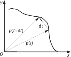
A parametric curve can be understood in terms of the evolution of a point (or a very small particle) as it moves along a 2-D space. Mathematically, the position of the particle on the plane can be expressed in terms of the position vector p(t) = [x(t) y(t)], where t is real and is called the parameter of the curve. For example, p(t) = [cos(t) sin(t)] specifies a trajectory of the unitary radius circle for 0 < t < 2π. In this interval, the curve starts at t = 0, defining a reference along its trajectory, and the parameter t corresponds to the angles with respect to the x-axis.
Consider now the situation depicted in Figure 6.3, which indicates the particle position with a given parameter value t, represented as p(t) = [x(t) y(t)], and the position at t + dt (i. e., p(t + dt)).
By relating these two positions as p(t + dt) = p(t) + dp, and assuming that the curve is differentiable, the speed of the particle with the parameter t is defined as
For instance, the speed of the parametric curve given by p (t) = [cos(t) sin(t)] is p′(t) = [x′(t)y′(t)] = [–sin(t) cos(t)].
6.2.2.3Regular Curve and Jordan Curve
When the speed of a parametric curve is never zero (the particle never stops), the curve is said to be a regular curve. When the curve never crosses itself, the curve is said to be a Jordan curve.
One of the most important properties of the speed of a regular parametric curve is the fact that it is a vector tangent to the curve at each of its points. The set of all possible tangent vectors to a curve is called a tangent field. Provided the curve is regular, it is possible to normalize its speed in order to obtain unit magnitudes for all the tangent vectors along the curve, which is given by
A same trace can be defined by many (actually an infinite number of) different parametric curves. A particularly important and useful parameterization is unitary magnitude speed. Such a curve is said to be parameterized by the arc length. It is easy to verify that, in this case,
That is, the parameter t corresponds to the arc length. Consequently, a curve can be parameterized by the arc length if and only if its tangent field has unitary magnitudes. The process of transforming the analytical equation of a curve into an arc length parameterization is called arc length reparameterization, which consists of expressing the parameter t as a function of the arc length, and substituting t in the original curve for this function.
6.3Description of Shape Property
One property of a shape region can be described by using different techniques/descriptors. This section discusses two important properties of shapes, for which people have designed/developed a number of different descriptors to depict them.
6.3.1Compactness Descriptors
Compactness is an important property of shapes, which is closely related to the elongation of a shape. Many different descriptors have been proposed to give people an idea of the compactness of a region.
6.3.1.1Form Factor (F)
The form factor of a region is computed from the perimeter B and area A of this region,
In continuous cases, the F value of a circular region is one and the F value of other forms of regions is greater than one. For digital images, it has been proven (see Haralick, 1992) that the F value of an octagon region achieves the minimum if the perimeter is computed according to 8-connectivity, while the F value of a diamond region achieves the minimum if the perimeter is computed according to 4-connectivity. In other words, which digital shape gives the minimum F value depends on whether the perimeter is computed as the number of its 4-neighboring border pixels or as the length of its border counting 1 for vertical or horizontal moves and for diagonal moves.
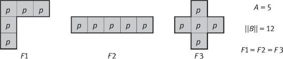
The form factor could describe, in a certain sense, the compactness of a region. However, in a number of situations, using only the form factor could not distinguish different shapes. One example is given in Figure 6.4, in which all three shapes have the same area (A = 5) and same perimeter (B = 12). According to eq. (6.4), they have the same form factors. However, it is easy to see from Figure 6.4 that these shapes are quite different.
6.3.1.2Sphericity (S)
Sphericity originates from 3-D, which is the ratio of the surface to the volume. In 2-D, it captures the shape information by the radius of the inscribed circle of object ri and the radius of the circumscribed circle rc, which is given by
One example is shown in Figure 6.5 (the centers of these circles do not generally coincide with each other or with the centroid).
The value of this descriptor attains its maximum for a circular object, and this value will decrease as the object extends in several directions.
6.3.1.3Circularity (C)
Circularity is another shape descriptor that can be defined by
where μR is the mean distance from the centroid of the region to the boundary pixels (see Figure 6.6) and σR is the standard variance of the distance from the centroid to the boundary pixels:
The value of this descriptor attains its maximum ∞ for a perfect circular object and will be less for more elongated objects.
Circularity has the following properties (Haralick, 1992):
1.As the digital shape becomes more circular, its value increases monotonically.
2.Its values for similar digital and continuous shapes are similar.
3.It is orientation and area independent.

6.3.1.4Eccentricity (E)
Eccentricity could also describe, in a certain sense, the compactness of a region. There are several formulas for computing eccentricity. For example, a simple method is to take the ratio of the diameter of the boundary to the length of the line (between two intersection points with a boundary), which is perpendicular to the diameter, as the eccentricity. However, such a boundary-based computation is quite sensitive to noise. Better methods for eccentricity take all the pixels that belong to the region into consideration.
In the following, an eccentricity measurement based on the moment of inertia is presented (Zhang, 1991a). Suppose a rigid body consists of N points, with masses m1, m2,..., mN and coordinates (x1, y1, z1), (x2, y2, z2), ..., (xN, yN, zN). The moment of inertia, I, of this rigid body around an axis L is
where di is the distance between the point mi and the rotation axis L. Without loss of generality, let L pass the origin of the coordinate system and have the direction cosines α, β, γ, eq. (6.9) can be rewritten as
where
are the moments of inertia of this rigid body around the x-axis, y-axis, and z-axis, respectively, and
are called the inertia products.
Equation (6.10) can be interpreted in a simple geometric manner. First, look at the following equation
It represents a second-order surface centered on the origin of the coordinate system. If the vector from the origin to this surface is r, which has the direction cosines α, β, γ, then taking eq. (6.10) into eq. (6.17) gives
Now let us consider the right side of eq. (6.18). As I is always greater than zero, r should be limited (i. e., the surface is closed). Since the surface under consideration is a second-order surface (conical surface), it must be an ellipsoid and can be called the ellipsoid of inertia. This ellipsoid has three orthogonal major axes. For a homogenous ellipsoid, any profile with two coplane axes is an ellipse, which can be called the ellipse of inertia. If taking a 2-D image as a planar rigid body, then, for each region in this image, a corresponding ellipse of inertia, which reveals the distribution of the points belonging to this region, can be obtained.
To determine the ellipse of inertia of a region, the directions and lengths of the two major axes of this region are required. The direction can be determined, for example, with the help of eigenvalues. Suppose the slopes of the two axes are k and l,
In addition, based on k and l, the lengths of the two axes of the ellipse of inertia, p and q, can be obtained by
The eccentricity of the region is just the ratio of p to q. Such defined eccentricity should be less sensitive to noise than boundary-based computations. It is easy to see that such a defined eccentricity would be invariant to the translation, rotation, and scaling of the region.
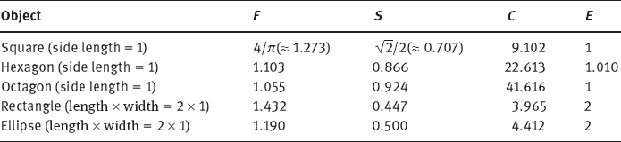
The values of the above-discussed descriptors F, S, C, and E for several common shapes are listed in Table 6.1.
The above descriptors are discussed in the continuous domain. Their computations for digital images are illustrated with the help of the following example sketches for a square in Figure 6.7. Figure 6.7(a, b) are for computing B and A in form factors (F), respectively. Figure 6.7(c, d) are for computing ri and rc in sphericity (S), respectively. Figure 6.7(e) are for computing μR in circularities (C). Figure 6.7(f–h) are for computing A, B, and H in eccentricities (E), respectively.
Table 6.1: The values of F, S, C, and E for several common shapes.

6.3.2Complexity Descriptors
Another important property of shapes is their complexity. Indeed, the classification of objects based on shape complexity arises in many different situations (Costa 2001). For instance, neurons have been organized into morphological classes by taking into account the complexity of their shapes (especially the dendritic tree). While complexity is a somewhat ambiguous concept, it is interesting to relate it to other geometric properties, such as spatial coverage. This concept, also known as the space-filling capability, indicates the capacity of a biological entity for sampling or interacting/filling the surrounding space. In other words, spatial coverage defines the shape interface with the external medium and determines important capabilities of the biological entity. For instance, a bacterium with a more complex shape (and hence a higher spatial coverage) will be more likely to find some food. At a larger spatial scale, the amount of water a tree root can drain is related to its respective spatial coverage of the surrounding soil. Yet another example of spatial coverage concerns the power of a neural cell to make synaptic contacts (see, e. g., Murray, 1995).
In brief, shape complexity is commonly related to spatial coverage in the sense that the more complex the shape, the larger its spatial covering capacity.
Unfortunately, though the term shape complexity has been widely used by scientists and other professionals, its precise definition does not exist yet. Instead, there are many different useful shape measurements that attempt to capture some aspects related to shape complexity. Some of them are listed in the following, in which B and A denote the shape perimeter and area, respectively.
6.3.2.1Simple Descriptors for Shape Complexity
1.Area to perimeter ratio, which is defined as A/B.
2.Thinness ratio, which is inversely proportional to the circular property of shape and defined as 4π(A/B2). The multiplying constant, 4π, is a normalization factor; hence, the thinness ratio is the inverse of the form factor.
3. which is related to the thinness ratio and to the circularity.
4.Rectangularity, which is defined by A/area (MER), where MER stands for minimum enclosing rectangle.
5.Mean distance to the boundary, which is defined by
6.Temperature, which is defined by T = log2[(2B)/(B–H)], where H is the perimeter of the shape convex hull (see Section 10.2). The contour temperature is defined based on a thermodynamic formalism.
6.3.2.2Histogram of Blurring Images
An interesting set of complexity measurements can be defined by the histogram analysis of blurred images. Recall that simple histogram measurements cannot be used as shape features because the histogram does not take into account the spatial distribution of the pixels, but only the gray-level frequencies.
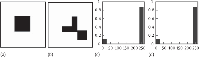
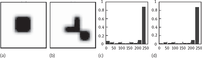
For instance, consider the two images in Figure 6.8(a, b), where two different shapes are presented in these two images, respectively. The two shapes have the same area and, as a result, the same number of black pixels. Therefore, they have identical histograms, which are shown in Figure 6.8(c, d), respectively. It is now to consider blurring these two shape images by an averaging filter. The results obtained are shown in Figure 6.9(a, b), respectively. These results are influenced by the original shapes in images, and thus, their corresponding image histograms become different, which are easily verified from Figure 6.9(c, d). Therefore, shape features can be defined by extracting information from the latter type of histograms (i. e., those obtained after image blurring).
A straightforward generalization of this idea is the definition of a multi-scale family of features (Costa 2001). These features can be calculated based on the convolution of the input image with a set of multi-scale Gaussians g(x, y, s) = exp[–(x2 + y2)/(2s2)]. Let f(x, y, s) = f(x, y) * g(x, y, s) be the family of the multi-scale (blurred) images indexed by the scale parameters and obtained by 2-D convolutions between f and g for each fixed value of the scale parameter. Examples of the multiscale histogram-based complexity features are listed in the following:
1.Multiscale entropy: It is defined as E(s) = –∑ipi(s) ln pi(s), where pi(s) is the relative frequency of the ith gray level in the blurred image f(x, y, s) for each value of s.
2.Multiscale standard deviation: It is defined as the square root of the variance of f(x, y, s) for each scale s. The variance itself can also be used as a feature.
6.3.2.3Fullness
There are certain relationships between the compactness and complexity of objects. In many cases, objects with relatively compact distribution often have relatively simple shapes.
Fullness in some senses reflects the compactness of the object, which takes into account the full extent of an object in a box around the object. One method to compute the fullness of an object is to calculate the ratio of the number of pixels belonging to the object with the number of pixels in the entire circumference box contains the object.
Example 6.1 Fullness of objects.
In Figure 6.10, there are two objects and their corresponding circumference boxes, respectively. These two objects have the same out-boundary, but the object in Figure 6.10(b) has a hole inside. The fullnesses of these two objects are 81/140 = 57.8% and 63/140 = 45%, respectively. By comprising the values of fullness, it is seen that the distribution of pixels in the object of Figure 6.10(a) is more concentrated than the distribution of pixels in the object of Figure 6.10(b). It seems that the density of pixel distribution in Figure 6.10(a) is bigger than that in Figure 6.10(b), while the complexity of the object of Figure 6.10(b) is higher that of the object in Figure 6.10(a).
The above obtained statistics is similar to statistics provided by histogram, which does not reflect the spatial distribution of information. It does not provide a general sense of shape information. To solve this problem, the lateral histogram of objects can be used. Here, the lateral histogram of X-coordinate is obtained by adding up the number of pixels along columns, while the lateral histogram of Y-coordinate is obtained by adding up the number of pixels along rows. The X-coordinate and Y-coordinate histograms obtained from Figure 6.10(a, b) are shown in Figure 6.11 up row and bottom row, respectively. The histograms of bottom row are both nonmonotonic histograms. There are obvious valleys in the middle, which are caused by the hole inside the object.![]()


6.4Technique-Based Descriptors
Different properties of a shape region can be described by using a particular technique, or by using several descriptors based on a particular representation. This section shows some examples.
6.4.1Polygonal Approximation-Based Shape Descriptors
A shape outline can be properly represented by a polygon (Section 3.2). Based on such a representation, various shape descriptors can be defined.
6.4.1.1Directly Computable Features
The following shape features can be extracted directly from the results of polygonal approximation by straightforward procedures.
1.The number of corners or vertices.
2.The angle and side statistics, such as their mean, median, variance, and moments.
3.The major and minor side lengths, side ratio, and angle ratio.
4.The ratio between the major angle and the sum of all angles.
5.The ratio between the standard deviations of sides and angles.
6.The mean absolute difference of the adjacent angles.
6.4.1.2Shape Numbers
Shape number is a descriptor for the boundary of an object based on chain codes. Although the first-order difference of a chain code is independent to rotation, in general, the coded boundary depends on the orientation of the image grid. One way to normalize the grid orientation is to align the chain-code grid with the sides of the basic rectangle. In practice, for a desired shape order, the rectangle of an order n, whose eccentricity best approximates that of the basic rectangle, is determined and this new rectangle is used to establish the grid size (see Section 3.5.2 for generating shape number).
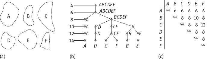
Based on the shape number, different shape regions can be compared. Suppose the similarity between two closed regions A and B is the maximum common shape number of the two corresponding shape numbers. For example, if S4(A) = S4(B), S6(A) = S6(B),..., Sk(A) = Sk(B), Sk+2(A) ≠ Sk+2(B),..., then the similarity between A and B is k, where S(·) represents the shape number and the subscript corresponds to the order. The self-similarity of a region is ∞.
The distance between two closed regions A and B is defined as the inverse of their similarity
It satisfies
One example of the shape number matching shape description is shown in Figure 6.12 (Ballard, 1982).
6.4.1.3Shape Signatures
One-dimensional signatures can be obtained from both contour/boundary-based and region-based shape representations. Contour-based signatures have been discussed in Section 3.2. The following brief discussions are for region-based signatures.
Region-based signatures use the whole shape information, instead of using only the shape boundary as in the contour-based approach. The basic idea is still to take the projection along different directions. By definition, a projection is not an information-preserving transformation. However, enough projections allow reconstruction of the boundary or even the region to any desired degree of accuracy (this is the basis for computer-assisted tomography as introduced in Chapter 5 of Volume I).
One example is shown in Figure 6.13. Two letters, S and Z, are in the forms of 7 × 5 dot-matrix representations, which are to be read automatically by scanning. The vertical projections are the same for these two letters. Therefore, a horizontal projection in addition would be necessary to eliminate the ambiguity.
This projection-based signature actually integrates the image pixel values along lines perpendicular to a reference orientation (e. g., projection signatures that are defined along the x and y axes). This concept is also closely related to the Hough transform.

There are many different ways to define signatures. It is important to emphasize that, as shape signatures describe shapes in terms of a 1-D signal, they also allow the application of 1-D signal processing techniques for shape analysis.
6.4.2Curvature-Based Shape Descriptors
The curvature is one of the most important features that can be extracted from contours. Strong biological motivation has been identified for studying the curvature, which is apparently an important clue explored by the human vision system.
6.4.2.1Curvature and Geometrical Aspects
As far as computational shape analysis is concerned, curvature plays an important role in the identification of many different geometric shape primitives. Table 6.2 summarizes some important geometrical aspects that can be characterized by considering curvatures (Levine, 1985).
6.4.2.2Discrete Curvature
In the discrete space, curvature commonly refers to the changes of direction within the discrete object under study. Hence, a discrete curvature only makes sense when it is possible to define an order for a sequence of discrete points. Therefore, the study of discrete curvature will be restricted to digital arcs and curves. The changes in directions will be measured via the angles made between the specific continuous segments defined by points on the discrete object in question.
Table 6.2: Curvatures and their geometrical aspects.
| Curvature | Geometrical Aspect |
| Curvature local absolute value maximum | Generic corner |
| Curvature local positive maximum | Convex corner |
| Curvature local negative minimum | Concave corner |
| Constant zero curvature | Straight line segment |
| Constant nonzero curvature | Circle segment |
| Zero crossing | Inflection point |
| Average high curvature in absolute or squared values | Shape complexity, related to the bending energy |
A formal definition of a discrete curvature is as follows (Marchand 2000). Given a set of discrete points P = {pi}i=0,…,n that defines a digital curve, ρk(pi), the k-order curvature of P at point pi ∈ P is given by ρk(pi) = |1 – cos θki|, in which (θki = angle (pi–k, pj, pi+k) is the angle made between the continuous segments [pi–k, pi] and [pi, pi+k], where k ∈ {i,...,n–i}.
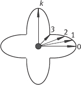
The integer order k is introduced to make the curvature less sensitive to local variations in the directions followed by the digital arc or curve. A discrete curvature of a high order will reflect more accurately the global curvature of the continuous object approximated by the set of discrete points. Figure 6.14 illustrates the process of calculating ρ3(p10), the third-order discrete curvature of the digital arc Ppq = {pi}i=0,...,17 at point p10.
Figure 6.15 displays the resulting curvature values obtained for successive instances of the order k (k = 1,..., 6) when using the digital arc presented in Figure 6.14. Clearly, the first-order curvature is not an accurate representation for discrete curvature since it only highlights local variations. This example also shows that as the order k increases, the curvature tends to illustrate the global behavior of the digital arc. The location of the peak (at point p8 or p9) corresponds to the place where a dramatic change in the global direction occurs in the digital arc.
6.4.2.3Curvature Computation
The curvature k(t) of a parametric curve c(t) = [x(t),y(t)] is defined as
It is clear from this equation that estimating the curvature involves the derivatives of x(t) and y(t), which is a problem where the contour is represented in a digital (spatially sampled) form. There are two basic approaches used to circumvent this problem.