
In many practical cases, a set of nine 5 × 5 convolution masks are used to compute the texture energy. To obtain these nine masks, the vectors L5, E5, S5, and R5 are used. L5 gives a center-weighted local average, E5 detects edges, S5 detects spots, and R5 detects ripples. The 2-D convolution masks are obtained by computing the outer product of each pair of vectors. For example, the mask is computed as the product of E5T and L5 as follows:
The first step is to remove the effect of illumination by moving a small window around the image, and subtracting the local average from each pixel, to produce a preprocessed image, in which the average intensity of each neighborhood is close to zero. The size of the window depends on the class of imagery. After the preprocessing, each of the 16 5×5 masks is applied to the preprocessed image, producing 16 filtered images. Let Fk(i, j) be the result of filtering the image with the kth mask at pixel (i, j). Then, the texture energy map Ek for filter k is defined by
Each texture energy map is a full image, representing the application of the kth mask to the input image.
Once the 16 energy maps are produced, certain symmetric pairs are combined to produce the nine final maps, replacing each pair with its average. For example, measures horizontal edge content, and measures vertical edge content. The average of these two maps measures total edge content. The nine resultant energy maps are
5.3Structural Approaches
The structural model regards the texture elements as repeating patterns and describes such patterns in terms of generating rules. Formally, these rules can be viewed as grammars. This model is best for describing textures where there is much regularity in the placement of elements and the texture is imaged at a high resolution (Ballard, 1982).
5.3.1Two Basic Components
To characterize a texture, the gray-level primitive properties must be characterized as well as the spatial relationships between them. This implies that texture-structure is really a two-layered structure. The first layer specifies the local properties that manifest themselves in gray-level primitives. The second layer specifies the organization among the gray-level primitives. Structural approaches for texture description are characterized by two components: Texture elements and arrangement rules.
5.3.1.1Texture Elements
A texture element is a connected component of an image, which can be characterized by a group of properties. The properties of texture regions depend on the property and number of texture elements. However, there is no commonly recognized set of texture elements. The simplest texture element is pixel, whose property is gray level. A little more complex texture element is a group of connected pixels with the same gray levels. Such a texture element can be described with the size, orientation, shape, and/or average gray level.
5.3.1.2Arrangement Rules
To describe texture, after obtaining the texture elements, it is needed to specify the arrangement rules. These rules are often defined by certain formal language/grammar.

First, look at a simple example. Consider the staircase pattern shown in Figure 5.5(a). Two primitive elements a and b are shown in Figure 5.5(b) and three rules can be defined.
1.S → aA indicates that the variable S, which is also a starting symbol, may be replaced by aA.
2.A → bS indicates that the variable A may be replaced by bS.
3.A → b indicates that the variable A may be replaced by constant b.
Now, if applying the first rule, it will get aA. If applying the second rule to A, it leads back to the first rule and the procedure can be repeated. However, if applying the third rule to A, the procedure will be terminated. The application of the three rules can generate the structure as shown in Figure 5.5(c).
The above method can be easily extended to describe more complex texture patterns. Suppose there are the following eight rewriting rules (a represents a pattern, b means shifting downwards, and c means shifting to the left).
1.S → aA indicates that the variable S, which is also a starting symbol, may be replaced by aA.
2.S → bA indicates that the variable S, which is also a starting symbol, may be replaced by bA.
3.S → cA indicates that the variable S, which is also a starting symbol, may be replaced by cA.
4.A → aS indicates that the variable A may be replaced by aS.
5.A → bS indicates that the variable A may be replaced by bS.
6.A → cS indicates that the variable A may be replaced by cS.
7.A → c indicates that the variable A may be replaced by constant c.
8.A → a indicates that the variable A may be replaced by constant a.
Then, different 2-D patterns will be generated.
For example, a is a disk-like pattern, as shown in Figure 5.6(a), then four consecutive applications of rules (1) followed by rule (8) will generate Figure 5.6(b). While the consecutive applications of rules (1), (4), (1), (5), (3), (6), (2), (4), and (8) will generate Figure 5.6(c).

5.3.2Typical Structural Methods
Based on the above-explained principles, many structural methods for texture analysis have been developed. Two of them are described in the following.
5.3.2.1Textures Tessellation
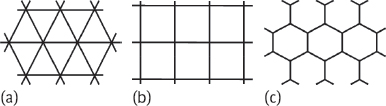
Highly patterned textures tessellate the plane in an ordered way, and thus, the different ways in which this can be done must be understood. In a regular tessellation, the polygons surrounding a vertex all have the same number of sides, as shown by Figure 5.7, where Figure 5.7(a) is for triangular, Figure 5.7(b) is for rectangular, and Figure 5.7(c) is for hexagonal (Ballard, 1982).
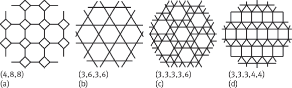
Semiregular tessellations have two kinds of polygons (differing in the number of sides) surrounding a vertex. Four semiregular tessellations of the plane are shown in Figure 5.8.
These tessellations are conveniently described by listing, in order, the number of sides of the polygons surrounding each vertex. Thus, a hexagonal tessellation is described by (6, 6, 6) and every vertex in the tessellation of Figure 5.9 can be denoted by the list (3, 12, 12). It is important to note that the tessellations of interest are those that describe the placement of primitives rather than the primitives themselves. When the primitives define a tessellation, the tessellation describing the primitive placement will be the dual of this graph as shown in Figure 5.9. Figure 5.9(a, c) shows primitive tessellation and placement tessellation, respectively. Figure 5.9(b) is the result of their combination.

5.3.2.2Voronoi Polygon
Suppose that a polygon has a set of already-extracted texture elements and that each one can be represented by a meaningful point, such as its centroid (Shapiro 2001). Let S be the set of these points. For any pair of points P and Q in S, the perpendicular bisector of the line joining them can be constructed. This perpendicular bisector divides the plane into two half planes, one of which is the set of points that are closer to P and the other of which is the set of points that are closer to Q. Let HQ(P) be the half plane that is closer to P with respect to the perpendicular bisector of P and Q. This process can be repeated for each point Q in S. The Voronoi polygon of P is the polygonal region consisting of all points that are closer to P than to any other point of S and is defined by
Figure 5.10 illustrates the Voronoi polygons for a set of circular texture elements. This pattern produces hexagonal polygons for internal texture elements, of which texture elements at the image boundary have various shapes.
5.3.3Local Binary Mode
LBP is a texture analysis operator. It is a texture metric defined with the help of local neighborhood. It belongs to the group of estimation method based on point samples, with the advantages of scale invariance, rotation invariance, and low computational complexity.

5.3.3.1Space LBP
The original LBP operator performs thresholding on the pixels in a 3 × 3 neighborhood in order, treats the result as a binary number and labels it for the center pixel. An example of a basic LBP operator is shown in Figure 5.11, where the left side is a texture image from which a 3 × 3 neighborhood is taken. The (count-clockwise) order of the pixels in the neighborhood is denoted by the numbers in parentheses, their values are represented by the following window. The result obtained by using 50 as the threshold value is a binary image. The binary number is 10111001 and the decimal value is 185. The histograms obtained from 256 different labels (for an 8-bit grayscale image) can be further used as the texture descriptors for image regions.
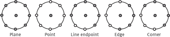
The basic LBP operator can be extended by using neighborhoods of different sizes. Neighborhoods can be circular, and for noninteger coordinate locations, the bilinear interpolation can be used to compute pixel values to eliminate restrictions on the neighborhood radius and the number of pixels in the neighborhood. Let (P, R) denote a rounded pixel neighborhood, where P represents the number of pixels in the neighborhood and R represents the radius of the circle. Figure 5.12 shows several examples of circular neighborhoods with their (P, R).
Another extension to the basic LBP operator is the uniform pattern. The pixels in a neighborhood are considered in a circular order, and if it contains up to two transitions from 0 to 1 or from 1 to 0, then the binary pattern is considered as uniform. The pattern 00000000 (0 transition) and pattern 11111001 (2 transitions) are uniform; while the pattern 10111001 (4 transitions) and pattern 10101010 (7 transitions) are not uniform. They have no obvious texture structure and can be regarded as noise. In the calculation of LBP labels, a separate label is used for each uniform pattern, and for all nonuniform models, the same label is commonly used. In this way, the antinoise ability can be enhanced. For example, when using the neighborhood (8, R), there are 256 patterns, 58 of which are uniform, so there are totally 59 labels. To sum up, can be used to represent such an LBP operator with uniform patterns.


Different local primitives can be obtained according to the labels of LBP, which correspond to different local texture structures. Figure 5.13 shows some (meaningful) examples where a hollow dot represents 1 and a solid dot represents 0.
Once the image fL(x, y) labeled with the LBP label is calculated, the LBP histogram can be defined as
where n is the number of distinct labels given by the LBP operator, I(z) is defined by
5.3.3.2Time-Space LBP
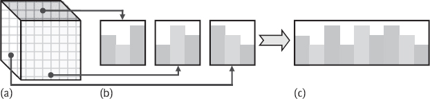
The original LBP operator can be extended to the time-space representation to perform dynamic texture analysis (DTA), which is the volume local binary pattern (VLBP) operator. It can be used for analyzing the dynamic changes of texture in 3-D(X, Y, T) space, including both motion and appearance. In the 3-D(X, Y, T) space, three sets of planes can be considered: XY, XT, YT. The three classes of LBP labels obtained are XY-LBP, XT-LBP, and YT-LBP, respectively. The first category contains spatial information, the latter two categories both contain time-space information. Three LBP histograms can be obtained from three categories of LBP labels, which can also be spanned together into a unified histogram. One example is shown in Figure 5.14. Figure 5.14(a) shows three planes of the dynamic texture. Figure 5.14(b) gives the LBP histogram for each plane. Figure 5.14(c) is the feature histogram after the stitching of three histograms.
Given a dynamic texture of X × Y × T: (xc ∈ {0,...,X – 1}, yc ∈ {0,...,Y – 1}, tc ∈ {0,..., T – 1}), the dynamic texture histogram can be written as:
where nj is the number of different labels produced by the LBP operator on the jth plane (j = 0 : XY, j = 1: XT and j = 2: YT), and fj(x, y, t) denotes the LBP code of the upper center pixel (x, y, t) on the jth plane.
For dynamic textures, it is not necessary to set the range of the time axis to be the same as the spatial axis. In other words, the distances between the temporal and spatial sampling points may be different in the XT and YT planes. More generally, the distances between the sample points on the XY, XT, and YT planes may be all different.
When it is necessary to compare dynamic textures that differ both in spatial and temporal scales, the histogram needs to be normalized to obtain a consistent description
In this normalized histogram, the description of the dynamic texture can be obtained efficiently based on LBP labels obtained from three different planes. The labels obtained from the XY plane contain information about the appearance, and the labels obtained from the XT and YT planes include the symbiotic statistics of motions in the horizontal and vertical directions. This histogram constitutes a global description for the dynamic texture with spatial and temporal characteristics. Because it has nothing to do with the absolute gray value, and only with the relative relationship between the local gray levels, so it will be stable when the illumination changes. The disadvantage of LBP features does come from the ignoring of the absolute gray level and the no distinction between the relative strength. Therefore, the noise may change the weak relative relation and change its texture.
5.4Spectral Approaches
Spectral approaches for texture analysis can be based on various spectra. Three of them, the Fourier spectrum, Bessel–Fourier spectrum, and Gabor spectrum are introduced below.
5.4.1Fourier Spectrum
The following three features of the Fourier spectrum are useful for texture descriptions (Gonzalez, 2002):
1.Prominent peaks in the spectrum give the principal direction of the texture patterns.
2.The location of the peaks in the frequency plane gives the fundamental spatial period of the pattern.
3.Eliminating any periodic component via filtering leaves nonperiodic image elements, which can then be described by statistical techniques.
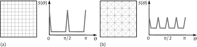
Expressing the spectrum in polar coordinates can yield a function S(r, θ), where S is the spectrum function and r and θ are the variables in this coordinate system. For each direction θ, S(r, θ) may be considered a 1-D function Sθ(r). Similarly, for each frequency r, Sr(θ) is a 1-D function. Analyzing Sθ(r) for a fixed value of θ yields the behavior of the spectrum (such as the presence of peaks) along a radial direction from the origin, whereas analyzing Sr(θ) for a fixed value of r yields the behavior along a circle centered on the origin.
A more global description is obtained by integrating these functions:
where R0 is the radius of a circle centered at the origin.
Figure 5.15 shows two texture regions and the plotted S(θ), and the orientation of the texture pattern can be quickly determined from their spectrum curves.
If a texture is spatially periodic or directional, its power spectrum will tend to have peaks for the corresponding spatial frequencies. These peaks can form the basis of the features as a pattern recognition discriminator. One way to define features is to partition the Fourier space into bins. Two kinds of bins, radial and angular (corresponding to the wedge filter and the ring filter, respectively) bins, are commonly used, as shown in Figure 5.16.
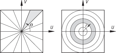
Radial features are given by (|F|2 is the Fourier power spectrum)
where the limits are defined by
Radial features are correlated with the texture coarseness. A smooth texture will have high values of R(r1, r2) for small radii, whereas a coarse and grainy texture will tend to have relatively higher values for larger radii.
Angular orientation features are given by
where the limits are defined by
Angular orientation features exploit the sensitivity of the power spectrum to the directionality of the texture. If a texture has many lines or edges in a given direction θ |F|2 will tend to have values clustered around the direction in the frequency space θ + π/2.
5.4.2Bessel-Fourier Spectrum
Variational calculus has been used to determine the Bessel–Fourier boundary function (Beddow, 1997)
where angle θ; Am,n, Bm,n are the Bessel–Fourier coefficients, Jm is the first kind mth order Bessel function, Zm,n is the zero root of the Bessel function, and Rv is the radius of the field of view.
The following descriptors for texture can be derived from eq. (5.46):
1.Bessel–Fourier coefficients.
2.Moments of the gray-level distribution (gray-level histogram).
3.Partial rotational symmetry: The texture is composed of discrete gray levels. An R-fold symmetry operation can be performed by comparing the gray-level value at G(R, θ) with that at G(R, θ + ∆θ). This provides the index Crt, the partial rotational symmetry index of the texture, as
where R = 1,2,..., Hm,nR2 = Am,nR2 + Bm,nR2.
4.Partial translational symmetry: A partial translational symmetry is recognized when the gray-level values are compared along the radius. So, G(R, θ) is compared with G(R + ∆R, θ). The partial translational symmetry index of the texture is 0 < Ctt < 1 and is defined as
5.Coarseness: The coarseness, Fcrs, is defined as the difference between the gray-level values of four neighboring points around a specific point (x, y).
Analysis has shown that the coarseness is related directly to the partial rotational and translational symmetries as given by
6.Contrast: In the case of a distribution in which the values of the variables are concentrated near the mean, the distribution is said to have a large kurtosis. The contrast, Fcon, is defined as the kurtosis by
where μ4 is the fourth moment of the gray-level distribution about the mean and σ2 is the variance.
7.Roughness: The roughness, Frou, is related to the contrast and coarseness as follows,
8.Regularity: The regularity, Freg, is a function of the variation of the textural elements over the image. It is defined by
An image with high rotational and high translational symmetries will have high regularity.
5.4.3Gabor Spectrum
The Fourier transform uses the entire image to compute the coefficients, while using a set of 2-D Gabor filters can decompose an image into a sequence of frequency bands (Gabor spectrum). The impulse response of the complex 2-D Gabor filter is the product of the Gaussian low-pass filter with a complex exponential (Theodoridis, 2003) as given by
where
and
It is thus clear that L′(x, y) is a version of the Gaussian L(x, y) that is spatially scaled and rotated by θ. The parameter σ is the spatial scaling parameter, which controls the width of the filter impulse response, and λ defines the aspect ratio of the filter that determines the directionality of the filter, that is no longer circularly symmetric.
The orientation angle θ is computed by
By varying the free parameters σ, λ, θ, w = (wx2 + wy2)1/2, the filters of arbitrary orientations and bandwidth characteristics are obtained.
Gabor filters come in pairs: One recovers the symmetric components in a particular direction, given by