
2Image Segmentation
Image segmentation is the first step of image analysis and is necessary for obtaining analysis results from objects in an image. In image segmentation, an image is divided into its constituent parts and those parts of interest (objects) are extracted for further analysis.
The sections of this chapter are arranged as follows:
Section 2.1 gives a formal definition of image segmentation. The image segmentation techniques are classified according to the definition. The classification methods presented here are general and essential and provide the foundation for the subsequent sections.
Section 2.2 introduces the basic knowledge of image segmentation and the basic principles and methods of various groups of segmentation techniques, such as parallel boundary, sequential boundary, parallel region, and sequential region ones.
Section 2.3 extends the basic segmentation techniques to solve the problem of image segmentation for different kinds of images and generalizes their principles to accomplish segmentation tasks that are more complicated.
Section 2.4 focuses on the evaluation of image segmentation algorithms and the comparison of different evaluation methods, which are at higher levels of image segmentation, respectively.
2.1Definition and Classification
Research on image segmentation has attracted much attention over the years and a large number (several thousands) of algorithms have been developed (Zhang, 2006b). Descriptions of an image generally refer to the significant parts of the image. Thus, an image description requires segmenting the image into such parts. Image segmentation is one of the most critical tasks in automatic image analysis and image recognition systems because the segmentation results will affect all thenceforth tasks, such as feature extraction and object classification.
2.1.1Definition of Segmentation
In image segmentation, an image is divided into different regions, each of which has certain properties (Fu, 1981). The aim of image segmentation is either to obtain a description of an image or to classify the image into meaningful classes. An example of the former is the description of an office scene. An example of the latter is the classification of an image-containing cancer cells.
Image segmentation can be defined more formally using mathematical tools and terms. To define image segmentation, the definition of the uniform predication is first discussed. Let S denote the grid of sample points in an image, that is, the set of points {(i, j)} , i = 1, 2, . . ., N, j = 1, 2, ..., M, where N and M are the number of pixels in the X and Y directions, respectively. Let T be a nonempty subset of S consisting of contiguous image points.
Then, a uniform predication P(T), a process that assigns the value of true or false to T, depends only on the properties related to the brightness matrix f(i, j) for the points of T. Furthermore, P has the property that if Z is a nonempty subset of T, then P(T) = true implies that P(Z) = true.
The uniformity predication P is a function with the following characteristics:
1.P assigns the value true or false to T, depending only on properties of the values of the image elements of T.
2.T ⊃ Z ∧ Z ≠ 0 ∧ P(T) = true ⇒ P(Z) = true; {(set Z is contained in set T) and (Z is a nonempty set) and (P(Y) is true) implies always (P(Z) is true)}.
3.T contains only one element: ⇒ P(T) = true.
Now consider the formal definition of image segmentation(Fu, 1981). A segmentation of the grid S for a uniformity predication P is to partition S into disjoint non-empty subsets S1, S2, ..., SN such that (where Si and Sj are adjacent):
1. (the union of all Si is (equivalent to) S}.
2.For all i and j and j ≠ j, it has Ri ∩ Rj = Ø.
3.P(Si) = true for i = 1, 2, ..., N.
4. = false for i ≠ j (the predication of the union of sets Si and Sj is false for i is not equal to j).
5.For i = 1, 2, ..., N, Si is a connected component.
The first condition implies that every image point must be in a region. This means that the segmentation algorithm should not be terminated until every point is processed. The second condition implies that the regions obtained by the segmentation should not overlap with each other. In other words, a pixel cannot belong to two different regions in the segmentation result. The third condition means that the pixels in a segmented region should have certain identical properties. The fourth condition indicates that the pixels in two different regions should have some distinguishable attributes. The fifth condition implies that regions must be connected components (i. e., comprising contiguous lattice points).
2.1.2Classification of Algorithms
Owing to the importance of image segmentation, much effort has been devoted to the segmentation process and technique development in the past few decades. This has already resulted in many (thousands) different algorithms, and the number of related algorithms is still increasing (Zhang, 2006b). A number of survey papers have been published (e. g., Fu, 1981; Haralick, 1985. Sahoo, 1988; Pal, 1993; Zhang, 2008d; 2015d).
A classification of algorithms is used to partition a set of algorithms into subsets. An appropriate algorithm classification scheme should satisfy the following four conditions (Zhang, 1993d):
1.Every algorithm must be in a group.
2.All groups together can include all algorithms.
3.The algorithms in the same group should have common properties.
4.The algorithms in different groups should have certain distinguishable properties each other.
Classification should be performed according to some classification criteria. The first two conditions imply that the classification criteria should be suitable for classifying all different algorithms. The last two conditions imply that the classification criteria should determine the representative properties of each algorithm group. Keeping these conditions in mind, the following two criteria appear to be suitable for the classification of segmentation algorithms.
The gray-level image segmentation is generally based on one of the two basic properties of the gray-level values in images: discontinuity and similarity(Fu, 1981). Therefore, two categories of algorithms can be distinguished: boundary-based algorithms that use the discontinuity property and region-based algorithms that use the similarity property. Evidently, such a classification satisfies the above four conditions. The region-based algorithms detect the object area explicitly while the boundary-based ones detect the object contours explicitly. Moreover, the object regions and their boundaries are complementary in images.
On the other hand, according to the processing strategy, segmentation algorithms can be divided into sequential algorithms and parallel algorithms. In the former, cues from earlier processing steps are used for the consequent steps. In the latter, all decisions are made independently and simultaneously. Though parallel methods can be implemented efficiently on certain computers, the sequential methods are normally more powerful for segmenting noisy images. The parallel and sequential strategies are also complementary from the processing point of view. Clearly, such a classification, along with the previous example, satisfies the four conditions mentioned above.
There is no conflict between the above two criteria. Combining both types of categorizations, four groups of segmentation algorithms can be determined (as shown in Table 2.1):
G1: Boundary-based parallel algorithms.
G2: Boundary-based sequential algorithms.
G3: Region-based parallel algorithms.
G4: Region-based sequential algorithms.
Table 2.1: Classification of segmentation techniques.
| Segmentation techniques | Parallel strategy | Sequential strategy |
| Boundary based | Group 1 (G1) | Group 2 (G2) |
| Region based | Group 3 (G3) | Group 4 (G4) |
Such a classification also satisfies the above four conditions mentioned in the beginning of this section. These four groups can contain all algorithms studied by Fu (1981) and Pal (1993). The edge-detection-based algorithms are either boundary-based parallel ones or boundary-based sequential ones depending on the processing strategy used in the edge linking or following. The thresholding and pixel classification algorithms are region-based and are normally carried out in parallel. Region extraction algorithms are also region-based but often work sequentially.
2.2Basic Technique Groups
According to Table 2.1, four groups of techniques can be identified. Some basic and typical algorithms from each group will be presented.
2.2.1Boundary-Based Parallel Algorithms
In practice, edge detection has been the first step of many image segmentation procedures. Edge detection is based on the detection of the discontinuity of the edges. An edge or boundary is the place where there is a more or less abrupt change in gray-levels. Some of the motivating factors of this approach are as follows:
1.Most of the information of an image lies in the boundaries between different regions.
2.Biological visual systems make use of edge detection, but not thresholding.
By a parallel solution to the edge detection problem, it means that the decision of whether or not a set of points is on an edge is made on the basis of the gray level of the set and some set of its neighbors. The decision is independent to the other sets of points that lie on an edge. So the edge detection operator in principle can be applied simultaneously everywhere in the image.
In boundary-based parallel algorithms, two processes are involved: The edge element extraction and the edge element combination (edge point detection and grouping).
2.2.1.1Edge Detectors
Since the edge in an image corresponds to the discontinuity in an image (e. g., the intensity surface of the underlying scene), the differential edge detector(DED) is popularly employed to detect edges. Though some particularly and sophisticatedly designed edge operators have been proposed (Canny, 1986), various simple DEDs such as the Sobel, Isotropic, Prewitt, and Roberts operators are still in wide use. These operators are implemented by mask convolutions. Figure 2.1 gives the two masks used for Sobel, Isotropic, and Prewitt edge detectors. For the Sobel detector,d = 2; for the Isotropic detector,d = 21/2; for the Prewitt detector,d = 1.
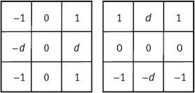

These operators are first-order DEDs and are commonly called gradient operators. In addition, the Laplacian operator, a second-order DED is also frequently employed in edge detection. Figure 2.2(a, b) gives two commonly used Laplacian masks.
These operators are conceptually well established and computationally simple. The computation of discrete differentiation can be easily made by convolution of the digital image with the masks. In addition, these operators have great potential for real-time implementation because the image can be processed in parallel, which is important, especially in computer vision applications.
The problems with edge detection techniques are that sometimes edges detected are not at the transition from one region to another and the detected edges often have gaps at places where the transitions between regions are not abrupt enough. Therefore, the detected edges may not necessarily form a set of closed connected curves that surround the connected regions.
2.2.1.2Hough Transform
The Hough transform is a global technique for edge connection. Its main advantage is that it is relatively unaffected by the gaps along boundaries and by the noise in images.
A general equation for a straight line is defined by
where p is the slope and q is the intercept. All lines pass through (x, y) satisfy eq. (2.1) in the XY plane. Now consider the parameter space PQ, in which a general equation for a straight line is

Consider Figure 2.3(a), where two points (xi, yi) and (xj, yj) are in a line, so they share the same parameter pair (p, q), which is a point in the parameter plane, as shown in Figure 2.3(b). A line in the XY plane corresponds to a point in the space PQ. Equivalently, a line in the parameter space PQ corresponds to a point in the XY plane.
The above duality is useful in transforming the problem of finding points lying on straight lines in the XY plane to the problem of finding a point that corresponds to those points, in the parameter space PQ. The latter problem can be solved by using an accumulative array as used in the Hough transform.
The process of the Hough transform consists of the following three steps:
1.Construct, in the parameter space, an accumulative array A(pmin: pmax, qmin: qmax).
2.For each point on the object (boundary), compute the parameters p and q, and then accumulate {A: A(p, q) = A(p, q) + 1}.
3.According to the maximum value in A, detect the reference point and determine the position of the object (boundary).
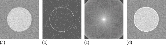
One example illustrating the results in different steps is presented in Figure 2.4, in which Figure 2.4(a) is an image with a circular object in the center, Figure 2.4(b) is its gradient image, Figure 2.4(c) is the image of accumulative array, and Figure 2.4(d) is the original image with detected boundary.
2.2.2Boundary-Based Sequential Algorithms
In a sequential solution to the edge detection problem, the result at a point is determined upon the results of the operator at previously examined points.
2.2.2.1Major Components
The major components of a sequential edge detection procedure include the following:
1.Select a good initial point. The performance of the entire procedure will depend on the choice of the initial point.
2.Determine the dependence structure, in which the results obtained at previously examined points affect both the choice of the next point to be examined and the result at the next point.
3.Determine a termination criterion to determine that the procedure is finished.
Many algorithms in this category have been proposed. A typical example is the snake, which is also called the active contour (Kass, 1988).
2.2.2.2Graph Search and Dynamic Programming
Graph search is a global approach combining edge detection with edge linking (Gonzalez, 2002). It represents the edge segments in the form of a graph and searches in the graph for low-cost paths, which correspond to edges/boundaries, using some heuristic information and dynamic programming techniques.
A graph G = (N, A) is a finite, nonempty set of nodes N, together with a set A of pairs of distinct elements (called arcs) of N. Each arc connects a node pair (ni, nj). A cost c(ni ,nj) can be associated with it. A sequence of nodes n1, n2,..., nK, with each node ni being a successor of node ni–1 is called a path from n1 to nK. The cost of the entire path is
The boundary between two 4-connected pixels is called an edge element. Figure 2.5 shows two examples of the edge element, one is the vertical edge element and the other is the horizontal edge element.

One image can be considered a graph where each pixel corresponds to a node and the relation between two pixels corresponds to an arc. The problem of finding a segment of a boundary can be formulated as a search of the minimal cost path in the graph. This can be accomplished with dynamic programming. Suppose the cost associated with two pixels p and q with gray levels of f(p) and f(q) is
where H is the highest gray level in the image.
The path detection algorithm is based on the maximization of the sum of the path’s merit coefficients. Usually, they are computed using a gradient operator, which replaces each element by some quantity related to the magnitude of the slope of the underlying intensity surface. The process of the graph search for the minimal cost path will be explained using the following example.
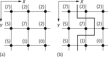
Consider a portion of the image as shown in Figure 2.6(a), where pixels are indicated by black discs and the numbers in the parentheses represent the gray levels of pixels. Here, H in eq. (2.4) is 7. Suppose a top-down path is expected. After checking each possible edge element, the minimal cost path corresponding to the sequence of the edge elements as shown by the bold line in Figure 2.6(b) can be found.
The graph for the above search process is shown in Figure 2.7.
Example 2.1 Practical implementation of the graph search process.
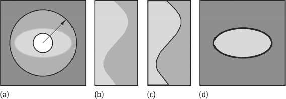
The boundary of objects in noisy two-dimensional (2-D) images may be detected with a state-space search technique such as dynamic programming. A region of interest, centered on the assumed boundary, is geometrically transformed and straightened into a rectangular matrix. Along the rows (of the matrix in the transform domain), merit coefficients are calculated. Dynamic programming is used to find the optimal path in the matrix, which is transformed back to the image domain as the object boundary (Figure 2.8).
Straightening the region of interest in a 3-D image can be accomplished in several ways. In general, the region of interest is resampled along scan lines, which form the rows of the coefficient matrix. The layout order of these rows in this matrix is not important, as long as two neighboring elements in the image domain are also neighbors in the resampled domain. The way the scan lines are located in the region of interest depends on the image (e.g., the scan lines are positioned perpendicular to the skeleton of the region of interest), while at the same time overlaps between scan lines are avoided. Another approach is to resample the data on a plane-by-plane basis. In this case, the number of planes in the image equal the number of planes in the resample matrix.![]()

2.2.3Region-based Parallel Algorithms
Thresholding or clustering(the latter is the multidimensional extension of the former) is a popular type of technique in the region-based parallel group. In its most general form, thresholding is described mathematically as follows:
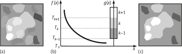
where (x, y) is the x and y coordinate of a pixel, g(x, y) is the segmented function, f(x, y) is the characteristic feature (e.g., gray level) function of (x, y). T0, ..., Tm are the threshold values, where T0 and Tm are the minimum and maximum threshold values, respectively. Finally, m is the number of distinct labels assigned to the segmented image (Figure 2.9).
The philosophy of this approach is basically a global one because some aggregate properties of the features are used. The similarity of the feature values in each class of a segmented region form a “mode” in the feature space. This technique is more resistant to noise than edge detection techniques. In addition, this technique produces closed boundaries though sometimes it is necessary to smooth some of the noisy boundaries.
Because the number of segments is not known, an unsupervised clustering scheme may not produce the right number of segments. Besides gray-level values, the features are generally image dependent and it is not clear how these features should be defined to produce good segmentation results. Furthermore, most researchers who have used this approach generally did not use the spatial information that is inherent in an image. Although attempts have been made to utilize the spatial information, the results so far are not better than those that do not use the information.
2.2.3.1Technique Classification
Determination of appropriate threshold values is the most important task involved in thresholding techniques. Threshold values have been determined in different techniques by using rather different criteria. Generally, the threshold T is a function of the form given by the following equation.
where f(x, y) is the gray level of the point located at (x, y) and g(x, y) denotes some local properties of this point. When T depends solely on f(x, y), the technique is point-dependent thresholding. When T depends on both f(x, y) and g(x, y), the technique is region-dependent thresholding. If, in addition, T depends also on the spatial coordinates x and y, then the technique will be coordinate-dependent thresholding.
A threshold operator T can also be viewed as a test involving a function T of the form T[x, y, N(x, y),f(x, y)], in which f(x, y) is the characteristic feature functions of (x, y) and N(x, y) denotes some local property (e. g., the average gray-level value over some neighbor pixels) of the point (x, y). Algorithms for thresholding can be divided into three types depending on the functional dependencies of the threshold operator T. When T depends only on f(x, y), the threshold is called a global threshold. If T depends on both f(x, y) and N(x, y), then it is called a local threshold. If T depends on the coordinate values (x, y) as well as on f(x, y) and N(x, y), then it is called a dynamic threshold.
In the case of variable shading and/or variable contrast over the image, one fixed global threshold for the whole image is not adequate. Coordinate-dependent techniques, which calculate thresholds for every pixel, may be necessary. The image can be divided into several subimages. Different threshold values for those subimages are determined first and then the threshold value for each pixel is determined by the interpolation of those subimage thresholds. In a typical technique, the whole image is divided into a number of overlapping sub-images. The histogram for each subimage is modeled by one or two Gaussian distributions depending on whether it is a uni-modal or a bi-modal. The thresholds for those subimages that have bi-modal distributions are calculated using the optimal threshold technique. Those threshold values are then used in bi-linear interpolation to obtain the thresholds for every pixel.
2.2.3.2Optimal Thresholding
Optimal thresholding is a typical technique used for segmentation. Suppose that an image contains two values combined with additive Gaussian noise. The mixture probability density function is
where μ1 and μ2 are the average values of the object and the background, respectively, and σ1 and σ2 are the standard deviation values of the object and the background, respectively. According to the definition of probability, P1 + P2 = 1. Therefore, there are five unknown parameters in eq. (2.7).
Now look at Figure 2.10, in which μ1 < μ2. Suppose a threshold T is determined, all pixels with a gray-level below T are considered to belong to the background, and all pixels with a gray-level above T are considered to belong to the object. The probabilities of classifying an object pixel as a background pixel and of classifying a background pixel as an object pixel are
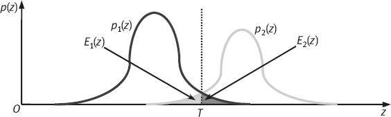
The overall probability of error is given by eq. (2.10):
In the case where both the object and the background have the same standard deviation values, the optimal threshold is
2.2.4Region-based Sequential Algorithms
In region-based segmentation techniques, the element of the operation is the region. The processes made on regions is either the splitting operation or the merging operation. A split, merge, and group(SMG) approach is described as follows, which consists of five phases executed in a sequential order.
1.Initialization phase
The image is divided into subimages, using a quad-tree (QT) structure (see Figure 2.11).
2.Merging phase
The homogeneity of the nodes of level Ls+1 is evaluated to see whether all sons on level Ls are homogeneous. If a node is homogeneous, the four sons are cut from the tree and the node becomes an end-node. This process is repeated for the level until no more merges can take place or the top level is reached (a homogeneous image).
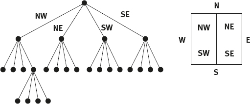
The in-homogeneous nodes on level Ls are processed. They are split into four sons that are added to the QT. The new end-nodes are then evaluated and are split again if necessary, until the quad-tree has homogeneous end-nodes only.
4.Conversion from QT to RAG (Region Adjacency Graph)
The QT, which emphasizes hierarchical inclusion relations, has been adopted to get the best of both the splitting and the merging approaches. Outside of this structure, however, it is still possible to merge different subimages that are adjacent but cannot be merged in the QT (because of an in-homogeneous father node or differing node levels). The region adjacency graph(RAG), in which adjacency relations are of primary concern, allows these merges to take place.
5.Grouping phase
The explicit neighbor relationships can be used to merge adjacent nodes that have a homogeneous union.
The path and the data structures are summarized in Figure 2.12.

2.3Extension and Generation
In the last section, several basic algorithms for segmenting 2-D gray-level images were described. Those algorithms can be extended to segment other types of images and their principles can be generalized to complete tasks that are more complicated. Note that the distinction between the parallel and sequential strategies also extends to the known segmentation algorithms for images of higher dimensionality. The extension of parallel methods to n-D is trivial (simple), as there is no interaction between assignment decisions of different image elements. When extending sequential methods, there is a choice between applying a (n-1)-D algorithm to each (hyper-) plane of the n-D image and a true n-D segmentation algorithm. The first approach means it has to use the information in the nth dimension explicitly to achieve an n-D segmentation result while an n-D algorithm uses the information implicitly. On the other hand, it is possible that an (n-1)-D approach will be less memory expensive and faster because the extra-dimensional information can be supplied more efficiently.
2.3.1Extending 2-D Algorithms to 3-D
A variety of imaging modalities make it possible to acquire true 3-D data. In these data, the value of a physical parameter is known for all spatial coordinates and thus it leads to a description f(x, y, z). 3-D segmentation is thus required and various algorithms have been developed. Many 3-D algorithms are obtained by extending the existing 2-D algorithms. According to the classifications shown in Table 2.1, several 3-D segmentation algorithms in different groups will be discussed.
2.3.1.13-D Differential Edge Detectors
In 3-D space, there are three types of neighborhoods. It can also say that in the 3-D space, there are three ways to define a neighbor: voxels with joint faces, joint edges, and joint corners (Jähne, 1997). These definitions result in a 6-neighborhood, an 18-neighborhood, and a 26-neighborhood.
Let x = (x0, ..., xn) be some point on an image lattice. The neighborhood of x is defined as
and the neighborhood of x is defined as
These neighbors determine the set of the lattice points within a radius ofi from the center point.
Let x = (x0, x1) be some point on a 2-D image lattice. The n-neighborhood of x, where n = 4, 8, is defined as
Let x = (x0, x1, x2) be some point on a 3-D image lattice. The n-neighborhood of x, where n = 6, 18, 26, is defined as
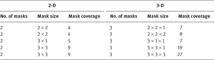
In digital images, differentiation is approximated by difference (e. g., by the convolution of images with discrete difference masks, normally in perpendicular directions). For 2-D detectors, two masks are used for x and y directions, respectively. For 3-D detectors, three convolution masks for the x, y, and z directions should be designed. In the 2-D space, most of the masks used are 2 × 2 or 3 × 3. The simplest method for designing 3-D masks is just to take 2-D masks and provide them with the information for the third dimension. For example, 3 × 3 masks in 2-D can be replaced by 3 × 3 × 1 masks in 3-D. When a local operator works on an image element, its masks also cover a number of neighboring elements. In the 3-D space, it is possible to choose the size of the neighborhoods. Table 2.2 shows some common examples of 2-D masks and 3-D masks.
Since most gradient operators are symmetric operators, their 3-D extensions can be obtained by the symmetric production of three respected masks. The convolution will be made with the x mask in the x–y plane, the y-mask in the y–z plane, and the z-mask in the z–x plane.
For example, the 2-D Sobel operator uses two 3 × 3 masks, while for the 3-D case, a straightforward extension gives the results shown in Figure 2.13(a), where three 3 × 3 × 1 masks for the three respective convolution planes are depicted. This extended 3-D Sobel operator uses 18 neighboring voxels of the central voxel. For the 26-neighborhood case, three 3 × 3 × 3 masks can be used. To be more accurate, the entry values of masks should be adapted according to the operators’ weighting policy. According to the Sobel’s weighting policy, the voxels close to the central one should have a heavier weight. Following this idea, the mask for calculating the difference along the x-axis is designed as shown in Figure 2.13(b). Other two masks are symmetric (Zhang, 1993c).

The Laplacian operator is a second-order derivative operator. In the 2-D space, the discrete analog of the Laplacian is often defined by the neighborhood that consists of the central pixel and its four horizontal and vertical neighbors. According to the linearity, this convolution mask can be decomposed into two masks, one for the x-direction and the other for the y-direction. Their responses are added to give the response of Laplacian. When extending this operator to the 3-D case, three such decomposed masks could be used. This corresponds to the 6-neighborhood example as shown in Figure 2.14(a). For the 18-neighborhood case, the mask shown in Figure 2.14(b) can be used. For the 26-neighborhood case, the mask would be like that shown in Figure 2.14(c).
2.3.1.23-D Thresholding Methods
Extending 2-D thresholding techniques to 3-D can be accomplished by using 3-D image concepts and by formulating the algorithms with these concepts. Instead of using the pixel in the 2-D image, the voxel is the 3-D image’s primitive. The gray-level value of a voxel located at (x, y, z) will be f(x, y, z) and its local properties will be represented by g(x, y, z), thus the 3-D corresponding equation of eq. (2.6) is (Zhang, 1990)
In the following, some special requirements to extend different groups of 2-D thresholding techniques will be discussed.
Point-Dependent Group: For a technique in point-dependent thresholding group, two process steps can be distinguished:
(i)The calculation of the gray-level histogram
(ii)The selection of the threshold values based on the histogram
When it goes from 2-D to 3-D using exclusively the individual pixel’s information, the only required modification is in the calculation of the histogram from a 3-D image, which is essentially a counting and addition process. As a 3-D summation can be divided into a serial of 2-D summations, this calculation can be accomplished by using the existing 2-D programs (the direct 3-D summation is also straightforward). The subsequent threshold selection based on the resulted histogram is the same as that derived in the 1-D space. In this case, real 3-D routines are not necessary to process 3-D images.
Region-Dependent Group: In addition to the calculation of the histogram from 3-D images, 3-D local operations are also needed for the region-dependent thresholding group of techniques. For example, besides the gray-level histogram, the filtered gray-level image or the edge value of the image is also necessary. Those operations, as the structural information of a 3-D image has been used, should be performed in the 3-D space. In other words, truly 3-D local operations in most cases require the implementation of the 3-D versions of 2-D local operators. Moreover, as it has more dimensions in space, the variety of local operators becomes even larger. For example, one voxel in the 3-D space can have 6-, 18-, or 26-nearest or immediate neighbors, instead of 4- or 8-neighbors for a 2-D pixel.
Coordinate-Dependent Group: Two consecutive process steps can be distinguished in the coordinate-dependent thresholding group. One threshold value for each subimage is first calculated, then all these values are interpolated to process the whole image. The threshold value for each subimage can be calculated using either point-dependent or region-dependent techniques. Therefore, respective 3-D processing algorithms may be necessary. Moreover, 3-D interpolation is required to obtain the threshold values for all voxels in the image based on the thresholds for the subimages.
2.3.1.33-D Split, Merge, and Group Approach
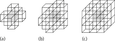
To adapt the SMG algorithm in last section to 3-D images, it is necessary to change the data structures that contain the 3-D information. The RAG structure can be left unchanged. The QT structure, however, depends on the image dimensionality. The 3-D equivalent is called an octree. The octree structure of a 3-D image is shown in Figure 2.15. Each father in this pyramidal structure has eight sons.
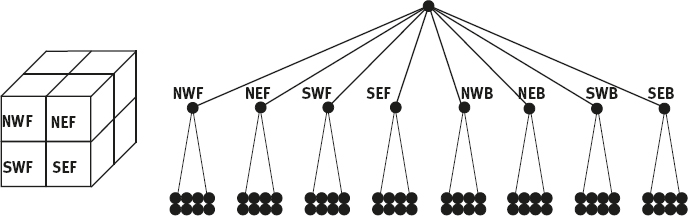
The initialization, split, and merge phases are analogous to those in the 2-D case because of the similarity of the quad-tree and the octree structures. The neighbor-finding technique also functions in the same way. Only the functions used to find the path in the tree from a node to its neighbor have to be adjusted for the 3-D case.
By simply replacing the quad-tree by an octree, the 3-D algorithm will be restricted to the image containing 2n × 2n × 2n voxels. In practice, 3-D images with lower z resolution are often encountered (anisotropic data). Three methods can be used to solve this problem (Strasters, 1991):
1.Adapt the image to fit into the octree structure, that is, increase the sampling density in the z direction or decrease the sampling density in the x and y directions.
2.Change the sequence of the data input, that is, input the image to the algorithm in such a way that it fits the octree structure.
3.Adapt the octree to make recursive splitting of the original image possible, that is, to allow all possible operations of the SMG algorithm on a 3-D image.
2.3.2Generalization of Some Techniques
Many of the above-described segmentation techniques could be generalized to fit various particular requirements in real applications. Two techniques are introduced in the following as examples.
2.3.2.1Subpixel Edge Detections
In many applications, the determination of the edge location at the pixel level is not enough. Results that are more accurate are required for registration, matching, and measurement. Some approaches to locate edge at the subpixel level are then proposed.
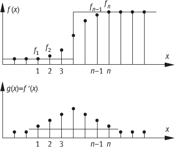
Moment Preserving: Consider a ramp edge as shown in the upper part of Figure 2.16, where the ramp values at each position 1, 2, ..., n-1, n are indicated by f1, f2, ··· , fn-1, fn. Edge detection is a process used to find a step edge (an idea edge), which in some sense fits best to the ramp edge. One approach is to keep the first three moments of the ramp and step edges equivalent to each other (moment preserving)(Tabatabai, 1984).
Consider the following formulation. The pth order of the moment (p = 1, 2, 3) of a signal f(x) is defined by (n is the number of pixels belonging to the edge)
It has been proven that mp and f(x) have a one-to-one correspondence. Let t be the number of pixels that have gray-level value b (background) and n–t be the number of pixels whose gray-level values are o (object). To keep the first three moments of two edges equivalent, the following three equations should be satisfied
where t is
in which
The edge is located at t + 0.5. This value is normally a real value that provides the subpixel accuracy.
Expectation of First-Order Derivatives: This approach computes the expectation of first-order derivatives of the input sequence and consists of the following steps (consider 1-D case) (Hu, 1992):
(i)For an image function f(x), compute the first derivative g(x) = |f′(x)|.
(ii)According to the value of g(x), determine the edge region (i. e., for a given threshold T determine the region [xi, xj], where g(x) > T, with 1 ≤ i, j ≤ n (Figure 2.16).
(iii)Compute the probability function p(x) of g(x):
(iv)Compute the expectation value E of g(x), which is taken as the location of the edge: