Chapter 6: Null Hypothesis Significance Testing
Statistics show that of those who contract the habit of eating, very few survive.
George Bernard Shaw
Biological Versus Statistical Ho
Introduction
We have now arrived at our last “theoretical” chapter before we start looking at specific case studies and tests. What is Null Hypothesis Significance Testing, also known affectionately as NHST? If we break the phrase apart, obviously we are talking about testing something (that is why it’s called “testing”). We are testing the significance of something, and there must be some criterion, if not multiple criteria, for assessing that significance. Hypotheses should be familiar to even the most basic of science majors. They are the proposed answers to our research questions around which our experimentation lies. But what does “null” mean, and more specifically, what is a null hypothesis?
Looking up “null” in the dictionary, one meaning that applies in this context is “without value, effect, consequence, or significance.”1 Of particular applicability here is “without effect.” Thus, the null hypothesis is the hypothesis of no effect, no difference, no change…in short, boring nothingness! It is usually what the scientist hopes to reject so that she can provide evidence for her hypothesis that there is an effect, a difference, a change…in short, that she has found a new result she can publish. (This is why one should “care” about NHST. It lies at the heart of data analysis.)
The null hypothesis (Ho) is in direct opposition to the research or alternative hypothesis (H1). Table 6.1 compares and contrasts these two. There may be more than one alternative hypothesis under consideration in any given line of research, but distinguishing between different alternative hypotheses falls into the arena of experimental design.
Table 6.1: Null vs. Research Hypothesis
|
Null Hypothesis (Ho) |
Research/Alternative Hypothesis (H1) |
|
No difference between populations |
The populations are different |
|
No relationship between two variables |
There is a relationship between two variables |
|
The particular intervention does not make a difference/has no effect |
The particular intervention does make a difference/has an effect |
Biological Versus Statistical Ho
At this point it is helpful to distinguish between two different types of null hypotheses in any given experiment because it will help in interpreting our results. When designing your experiment, your research question should lead you to formulate a biological null hypothesis, which defines the absence of an effect in biological terms specific to what you are investigating. The biological null hypothesis frequently needs to be translated into an appropriate statistical null hypothesis that then enables you to evaluate the biological Ho. The statistical Ho is formulated in terms of the statistical metric or metrics that will be evaluated by your statistical test.
For example, let’s go back to our example of geckos climbing walls as a function of temperature. Your research question is something along of the lines of “does temperature affect the rate at which geckos climb walls?” Your biological Ho is: temperature does not affect the rate at which geckos climb walls. This is the question that you, as a biologist, are really interested in. But when you go into the lab (or out in the gecko habitat) and collect your data, you now have two or more populations of rates at a minimum of two temperatures. How do you answer your question objectively with this data? The statistical Ho is what will guide you to your conclusion. The best statistical Ho is that there is no difference in the mean rate of climbing walls at the different temperatures. In order to answer the biological question, we calculate the metric of the mean of the rate populations and compare them for significant differences with a statistical test.2
NHST Rationale
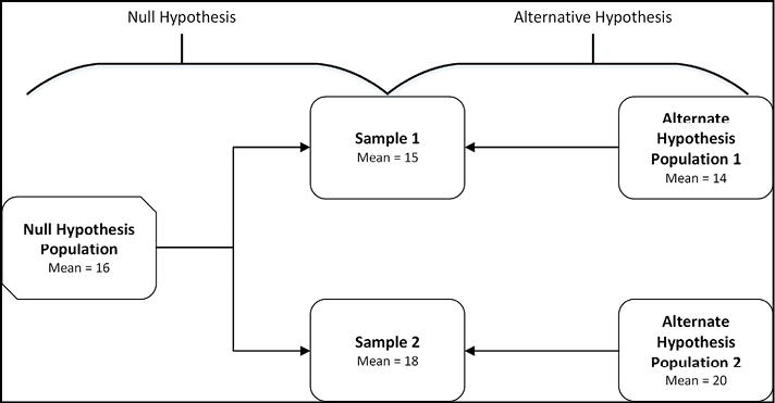
Null Hypothesis Significance Testing (NHST) has a specific rationale as illustrated in Figure 6.1. You have measured the same thing on two different populations and obtained a mean of 15 in one population and a mean of 18 in the other. The null hypothesis says the samples come from the same population and are different just by chance due to the inherent variation in the system (and possibly in your measurement instrumentation). This is depicted on the left side of Figure 6.1. Alternatively, on the right side of Figure 6.1, the two samples might come from two distinct populations and are not different by chance but because they are, in fact, different populations. So, which is it?
Figure 6.1: The Alternative Hypotheses of NHST
The application of the NHST rationale can be done in four steps:
1. Construct your null hypotheses (biological statistical)
2. Choose a critical significance level for the p-value (0.05 is the default; more on this in a moment)
3. Calculate a statistic (JMP does this for you, which is why we love software)
4. Reject or fail to reject the null hypotheses based on the p-value associated with the calculated statistic
p-Values
Steps 2 and 4 use this metric call the p-value. Just what is a p-value? The more statistical definition is the probability of getting a value for the test statistic equal to or more extreme than that calculated3 for the Ho if the null hypothesis is true. Since most of us will have trouble parsing that definition, another way of defining the p-value is the probability that the observed difference is due to chance alone. Or, to put it yet another way, from the perspective of very low p-values, the p-value is the probability that you mistakenly rejected a true null hypothesis.
The traditional critical significant level of 0.05 is just that, tradition. It has no basis in theory, only in practice. You are saying that as long as the p-value is ≤ 0.05, the maximum probability of rejecting a true hypothesis that you will accept is 5% (or a 95% confidence level). We could just as easily have said that you really wanted to be much more convinced and accept an even smaller probability of being wrong, so you set the critical significance level to 0.01 (a 1% chance of error, or 99% confidence). Conversely, if the nature of your investigation is such that you are willing to accept a higher chance of error, then you could set it to 0.10 (a 10% chance of error, or 90% confidence). Or you can set it at any other value you think appropriate. However, the traditional 0.05 will be used throughout the rest of this work for simplicity’s sake.
p-Value Interpretation
Interpreting the p-value is straightforward once you have set it. When p < 0.05, we say there is a statistically significant difference and we reject the null hypothesis. One way to remember this is to learn the phrase, “If p is low, the null must go.” When p is > 0.05, we fail to reject the null hypothesis. Notice that we are not “accepting” the null hypothesis. In part, this is because failing to reject the null hypothesis does not mean that the null hypothesis is correct, only that there is not enough evidence to reject it. Remember we are in the foggy realm of probabilities, and unless you are omniscient, the null hypothesis can never be disproved. You can only say whether there is enough evidence to support it. A key axiom to remember: The absence of evidence is not evidence of absence.
A Tale of Tails…
Another aspect to be aware of is the distinction between one- and two-tailed tests. P-values are calculated for both, but what do they mean? What is the difference? Let’s refresh our little gray cells on the shape of a normal distribution with Figure 6.2.
Figure 6.2: A Normal Distribution Revisited
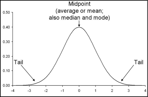
Notice that the normal distribution has two tails, one on either end of the curve. They are called tails because they are obviously shrinking in size as fewer and fewer members of the population are found in these parts of the curve, so they sort of look like tails. (Also, maybe the statistician who named them was an animal lover?!?) A two-tail test is one that simply wants to determine whether a difference exists between two populations regardless of the direction. That is, it is irrelevant to the goal of the experiment whether population A is greater than or less than population B, you just want to know whether they are different. One-tail tests, then, are for directional hypotheses where you want to know specifically if population A is greater than (or less than) population B. JMP provides p-values for all three types of tests: two-tail, and one-tail in either direction. This should be clearer after we walk through a sample case study at the end of this chapter.
Error Types
The significance level of p-values is usually set with reference to this mysterious Greek letter alpha, α. Alpha is used to designate what is called a Type I error, defined as incorrectly rejecting a true null hypothesis. You can call this a false positive error because when you reject a null hypothesis, you are accepting the alternative hypothesis as true and saying there is something going on (for example, a difference or relationship is present) when in fact it is not. Sort of like a doctor telling a male patient that he is pregnant.
There is another type of error the analyst can make. If you do not reject a false null hypothesis, you have committed a Type II error (often referred to as β), or accepted a false negative. To use our previous example, it would be like a doctor telling an obviously pregnant female patient that, no, you are not pregnant! Table 6.2 shows the various options to clarify.
Table 6.2: Error Types
|
Conclusion: REJECT |
Conclusion: DO NOT REJECT Null Hypothesis |
|
|
Null Hypothesis is TRUE (no effect exists) |
Type I error (α) |
No error (correct conclusion) |
|
Null Hypothesis is FALSE (an effect does exist) |
No error (correct conclusion) |
Type II error (β) |
Perhaps the bottom line of these concepts that the biologist should always keep in mind is that there is always a finite chance, however small, that your experiment will find a statistically significant difference when none exists.
A Case Study in JMP
Mild-to-severe chronic obstructive pulmonary disease (COPD) usually reduces the ability to engage in physical activity for those suffering from this ailment. To determine if this actually is the case, athletic performance was measured by seeing how far (in meters) individuals could walk in six minutes. A group of COPD patients was compared to age- and sex-matched controls with no disease.
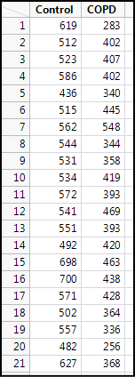
What is the biological null hypothesis? Simply that COPD has no effect on the distance walked compared to the controls. How do we translate this into a statistical null hypothesis? Well, what type of data do we have? (See Figure 6.3.) Each group has a set of continuous data of the distances walked by each subject in the group. The best way to summarize these two groups would be to find the central tendency, that is, the mean. So, our objective is to compare the two groups and the easiest way to compare them is to compare the means. Therefore, our statistical null hypothesis is that there is no difference in the mean distance walked of the COPD and control groups. Notice two things about this process. We have employed the Y.O.D. part of our Y.O.D.A. strategy, and the formulation of our two types of null hypotheses worked synergistically to identify the overall objective and how we were going to get there. This is one of the advantages of thinking in terms of null hypotheses.
Figure 6.3: Raw Data for the Case Study
This type of analysis is a standard t test, which will be covered more extensively in Chapter 9. For now, we will work through the example in JMP to see how to apply the concepts described in this chapter. Trust me…by the end of the book, you will know more than you probably want to know about the t test, but you will be prepared to use it correctly and interpret it easily.
The data in Figure 6.3 is presented in the form in which it was probably collected, and most likely in an Excel table (it’s already in JMP in this figure, but transfer between JMP and Excel has been made incredibly easy, so no worries there). Each column can be summarized in this format, but the actual comparison requires a reconfiguration of the data. Think in terms of the independent and dependent variables of the experimental design. The independent variable is not the control, but rather the group identity. The dependent variable is the distance walked. Thus, the independent variable is actually across the top of this initial JMP data table in the column headings!
JMP allows for this reconfiguration in the Table menu. It is the Stacking option and the filled-out menu is in Figure 6.4.
Figure 6.4: Stacking the Data
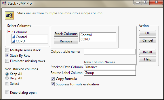
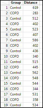
The two columns have been moved over into the Stack Columns box, and the New Column Names entered into the appropriate boxes. Clicking OK yields the new data table (neatly preserving the initial data) seen in Figure 6.5.
Figure 6.5: New Stacked Data Ready for Analysis
Now open the Fit Y by X platform in the Analyze menu and put the Group as the X, Factor and the Distance as the Y, Response (Figure 6.6), and click OK. Depending on the settings in your preferences, you should see something like Figure 6.7. (Don’t worry if your results look different; how to get there will be explained in Chapter 9 when we cover this test in more detail.)
Figure 6.6: Fit Y by X Dialog Box Filled Out for the Analysis
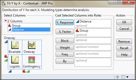
Figure 6.7: Analysis Results
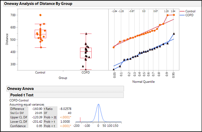
Looking at this output, JMP provides the graph that immediately lets us see that the COPD population is lower than the control population, but there is some overlap. The normal quantile plots allow us to evaluate the assumptions of a t test, but more on that in Chapter 9. For now, we want to focus on the t test table in which we find the more useful objective information. In the left column, we can note that the test execution has subtracted the control mean from the COPD mean to get the Difference. JMP then provides the Standard Error of the Difference (review Chapter 5 if you are unclear on what the Standard Error represents). It then provides the confidence limits (CL) and the significance level of those CL for the difference, which defaults to 95% (or 0.95). This characterizes the difference between the means of these two groups/populations.
The question at hand is whether this difference is significant, that is, is it greater than expected based on chance alone? This is where the metrics in the right column come in. Remember that statistical tests compute some metric to which the p-value is associated. In this case, the t ratio is calculated with the degrees of freedom (DF) as shown (using an equation of which we are gloriously ignorant and pragmatically don’t want to know because the software does it all). That doesn’t help us much because we don’t know what value to compare the t ratio to in order to make any kind of determination. Since we just want to know if there is a difference, the two-tailed p-value will be sufficient for the purposes of this analysis, so we can look at the Prob > |t| value of < .0001. This value tells us the probability of seeing a t ratio this large by chance alone is really, really small if the null hypothesis were true. Therefore, we can safely reject the null hypothesis of no difference between the means and conclude that there is a statistically significant difference in the means of these specific populations. This latter caveat should always be kept in mind since we only have a sample of the total population for each condition.
Endnotes
1 Definition of “null” from www.Dictionary.com; accessed 10 July 2017.; accessed 10 July 2017.
2 In the medical field, the biological null hypothesis may be referred to as the clinical null hypothesis. The presence or absence of statistical significance may be referred to as clinical significance.
3 Back in the Dark Ages, before the dawn of computers, these critical values would be laboriously hand calculated and tabulated in monster tables along with their associated p values. Yet another reason to rejoice that we have computers and software like JMP in these enlightened times!