Chapter 15: Modeling Trends: Generalized Linear Models

A theory has only the alternative of being right or wrong. A model has a third possibility: it may be right, but irrelevant.

Manfred Eigen

Introduction

What Are Generalized Linear Models?

The Underlying Forms

Why Use Generalized Linear Models?

How to Use Generalized Linear Models

The General Linear Model

GLM Assumptions

Reading the Output: Questions Answered

Is Weight a Function of… (a GLM Example)

Binomial Generalized Linear Models

Assumptions of the Binomial GLZM

How Severe Is It?

Poisson Generalized Linear Models

Poisson Distributions

Counting Nodes

Introduction

Chapters 11–14 have dealt with the right branch of our master flowchart (Figure 2.2), and we are still dealing with the main objective of that branch of the flow here in this chapter. That is to say, our goal continues to be determining the presence and nature of any associations between variables. But we have made some assumptions along the way, and we now turn our attention to some methods where those assumptions are not necessary to address situations where we still have data to torture analyze to make inferences about our biological situation.

What Are Generalized Linear Models?

An increasingly popular framework approach to modeling that does not require the data to meet the usual requirements of traditional linear models is found in the generalized linear model approach. The traditional linear models assume continuous response variables that are normally distributed as well as constant variance across all observations. There are many situations within biology where these are not true. For example, what if the variable you want to model1 is count or frequency data? These usually display a Poisson distribution2 rather than a normal distribution. What about proportions where the observed values are restricted to the range of 0 to 1? There are likewise many situations where the response of interest is binomial (for example, diseased versus healthy, or alive versus dead, or male versus female, and so on). For situations like these, we can use generalized linear models as we shall see in this chapter.

The Underlying Forms

Notice that I said “forms” and not “formulas.” We will continue to avoid the underlying mathematics of these methods in our pursuit of a practical working knowledge of how to use them appropriately. However, there is some basic understanding that will help us achieve this goal. There are three components to a generalized linear model: random, systematic, and link.

There is a random component that is based on the probability distribution of the response variable being modeled. These distributions can be normal, binomial, Poisson, or exponential. We will concern ourselves with the first three here, and the Generalized Linear Model Personality in the Fit Model platform will need to be told which one you want to use for your modeling.

The second component is a systematic component that is a linear combination of the independent variables in the model (thus generalized linear models). This component helps estimate the regression parameters using a method called maximum likelihood rather than the least squares method that we have been using.

These two components are connected by the third component, the link function. The link function helps define how the response variable is related to the explanatory variable(s). Specific link functions are normally associated with specific probability distributions of the random component, but the model framework allows for flexibility in which link function to use in the modeling efforts. Table 15.1 delineates the components of the most commonly used generalized linear models with the link functions identified.

Table 15.1: Generalized Linear Model Components

Random	Systematic	Default Link Function
Normal	Continuous	Identity
Normal	Categorical	Identity
Normal	Mixed3	Identity
Binomial	Mixed	Logit
Poisson	Categorical	Log
Poisson	Mixed	Log

Why Use Generalized Linear Models?

We have already seen ways to model binomial data (nominal logistic regression) and normally distributed data (standard least squares models), so why use generalized linear models instead? The easiest reason to understand is the application to binomial and Poisson data where the response does not need to be transformed to create normally distributed data. However, the ability to modify the link function to other than the default choice (which JMP gives you by default) gives more flexibility in modeling. A third reason is that these models require only one procedure in a software application to capture all the modeling possibilities (in other words, you find them all under one menu option in the software instead of having to hunt them down; of course, that is also a function of how good the software developers are in creating the user interface, but we won’t go there). There are other statistical and mathematical reasons that go beyond the scope of this course, at least that’s my story and I’m stickin’ to it! (Translation: I don’t understand them myself and neither would you unless you are a math major or a statistical genius! It is enough for me to know such reasons exist, and I will trust the statisticians that say so.)

How to Use Generalized Linear Models

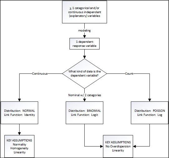
The Fit Model platform output provides the same statistics as we have seen before for the summarization and evaluation of different models. Thus, parameter estimates, standard errors, goodness-of-fit statistics, and so on, are provided and interpreted as we have been doing. All the new things are “under the hood” and invisible to the user. The goodness-of-fit statistics are particularly important since a primary aspect of modeling is the selection and comparison of various combinations of explanatory variables4 in the search for the best fit to the data.5 Figure 15.1 shows how to select which model to use for any given data set. Walking through this flowchart will be the rest of this chapter.

Figure 15.1: The Generalized Linear Model Flowchart

The General Linear Model

When the response being modeled is expected to have a reasonably normal distribution of continuous data, the generalized linear model is called the general linear model (GLM). (Yes, I know this is confusing, but I didn’t come up with the names; but at least it will make sure you are awake!) This is the left branch of our flowchart (Figure 15.1). GLM does not work well with small sample sizes, although how small is too small has no clear answer.

GLM Assumptions

The flowchart indicates three assumptions for the general linear model: normality, homogeneity, and linearity. Before we look at an example, we should understand what these assumptions are.

The first is normality, but it is the normality of the error or residuals. A normal quantile plot of the residuals would be the best way to evaluate this, but this platform does not provide one. You will have to save the residuals to the data table and then evaluate the distribution of that column to determine whether this criterion is met using the methods discussed in Chapter 4.

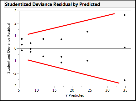
The second assumption is listed as homogeneity, and this is the homogeneity of the residuals. In other words, when plotted against the predicted values of the model, the residuals should display an even “shotgun” pattern above and below the zero line with no particular shape (see Figure 15.2), indicating a relatively constant variation across the range of predicted values. A lack of homogeneity is evidenced by a funnel shape to the residual cloud. (See Figure 15.3.)

Figure 15.2: Random Residuals = Homogeneous and Linear

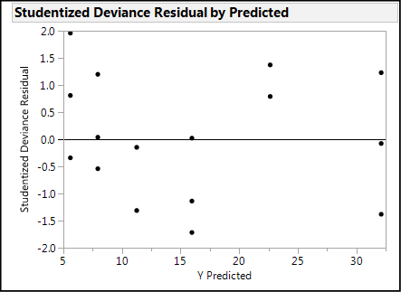
Figure 15.3: Non-homogenous Residuals

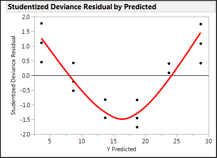
The third assumption is linearity, and this also refers to the residuals. Linearity is also evidenced by a lack of a pattern (other than the proverbial shotgun blast of randomness) as seen in Figure 15.2. Nonlinear residuals will show a shape other than (or perhaps in addition to) a funnel as shown in Figure 15.4. Nonlinearity is often caused by a failure to include significant interactions in the model. (More on interactions and DOE will be discussed in Chapter 16.)

Figure 15.4: Nonlinear Residuals…NOT a Smiley Face!

Reading the Output: Questions Answered

Generally, there are three fundamental questions the analyst wants to answer with this modeling. First, does this model describe a significant amount of the variation in the response variable? The Whole Model Test chi-square p-value answers this for the overall model. There are also chi-square p-values associated with each effect in the model (Effect Summary and Effect Tests output) that indicate the relative importance of the individual variables to the overall response.

If the answer to the first question is yes, that is, our whole model is statistically significant, then the second question can be addressed: what is the best linear model based on which explanatory variable(s)? The aforementioned p-values determine which variables to include, and then JMP provides the Parameter Estimates with their 95% confidence ranges that it then uses in the Profiler (or Save Formulas) for prediction purposes.

The third related question to address comes into play when comparing models: how good is the model compared to other possible models? Here we look more closely at the AICc or BIC values,6 remembering that the BIC generally penalizes models that have more parameters than does the AICc, so it will generally lead to the selection of models with fewer parameters. In both cases, the smaller the value, the better the fit.

Is Weight a Function of… (a GLM Example)

For our example of a GLM, open the Big Class.jmp sample data file from the files that come with JMP (Help  Sample Data  “Open the Popular Big Class.jmp Sample Data Table” button). Here we have the name, age, sex, height, and weight of 40 individuals. Our biological question is, can we predict the approximate weight of an individual based on knowledge of their age, sex, and height? This is just another way of asking if there is an association between these four variables that is strong enough to allow for prediction of weight using the other three variables.

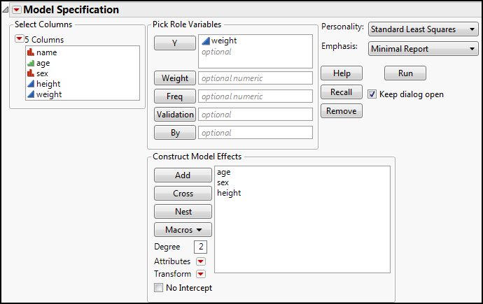
For comparison, first open the Fit Model platform and use the Standard Least Squares personality, but change the Emphasis to Minimal Report, then click Run (Figure 15.5).

Figure 15.5: Fit Model with SLS

This should give the output in Figure 15.6 (with the Profiler turned on from the Little Red Triangle menu).

Figure 15.6: Fit Model SLS Output

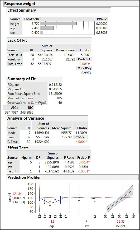
Reading down the output, we first see (Effect Summary) that height is a very significant contributor to weight (p < 0.0001; not a surprising biological outcome). Age is less of a contributor, but still statistically significant (p = 0.0340), and sex does not contribute significantly at all (p = 0.3801). There is a significant lack of fit; however, p = 0.0083, indicating that the model is not a good as it could be. Nevertheless, the RSquare value indicates we are accounting for a full 71% of the variation in the weight with these three variables, and the ANOVA output has a p-value of < 0.0001, so the model as a whole is significant. The Prediction Profiler shows the error bars for the nominal variables and a 95% confidence range around the continuous height variable, allowing for a visual assessment of the model. At the settings shown, the weight is predicted to be about 121, with a possible range of 109–134.7

Now, go back to Analyze  Fit Model. Enter the same variables in the same places, but this time change the Personality to Generalized Linear Model and set the Distribution to Normal (Figure 15.7).

Figure 15.7: Fit Model with Generalized Linear Model

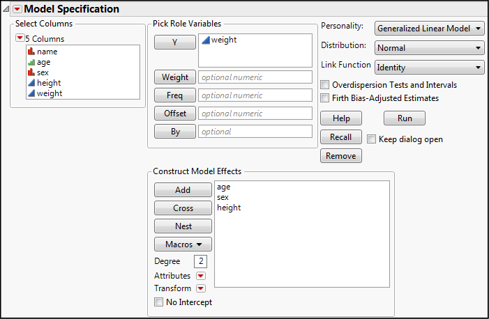
JMP defaults to the usual Link Function automatically, but this can be changed if the analyst has a reason to believe a different function will work better (or if it is desired to see if a different link function will work better). Clicking Run yields the output in Figure 15.8.

Figure 15.8: GLM Output

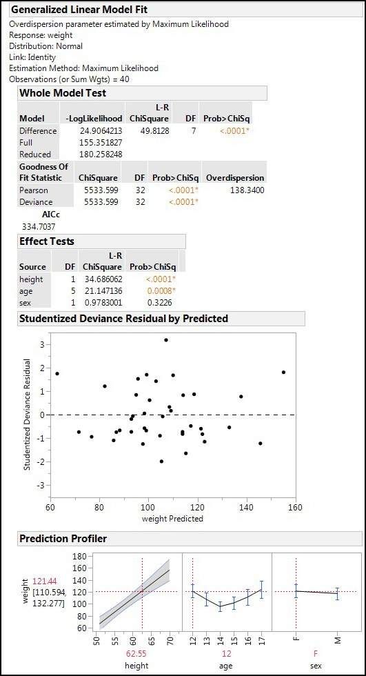
The output first provides a summary of the settings used for the analysis, and then we see that the Whole Model Test by this method also shows that a significant model has been constructed with these variables (p < 0.0001). In this case, the goodness of fit metric is the overdispersion rather than a lack of fit metric (same idea, different math and method). The greater the overdispersion, the greater the model’s variability compared to that expected based on the theoretical distribution. One could also say the greater the overdispersion, the greater the lack of fit.

The Effect Tests show the same results as we saw with standard least squares, but with slightly different p-values. The residual plot shows no non-homogeneity or non-linearity, so those assumptions of the GLM have been met. Lastly in this output, the Prediction Profiler presents the same picture as seen before for each of the variables, although the 95% confidence range for the predicted weight is slightly tighter with the GLM results (111–132 versus the 109–134 with the SLS output).

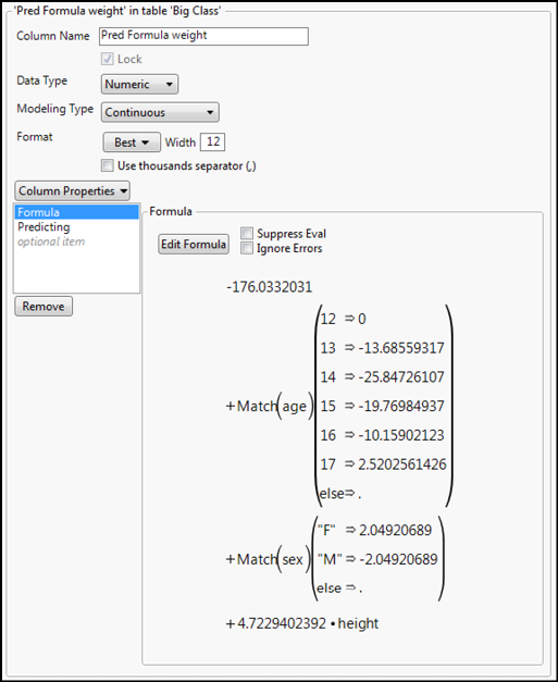
To check the normality assumption, click the Little Red Triangle for the Generalized Linear Model Fit, go down to the Save Columns menu and select Studentized Deviance Residuals (Figure 15.10). This will create a new column in the data table of those residuals. Notice the Prediction Formula can also be saved to the data table for predicting weight values with this model, along with the Mean Confidence Interval for the 95% confidence range of the weights already in the table. (Alas and forsooth, it is not a formula, so it cannot predict for unknown values.) An interesting benefit of saving the Prediction Formula is the ability to see the actual formula used by going to the Column Information of that column and looking at the formula (Figure 15.9).

Figure 15.9: The Prediction Formula

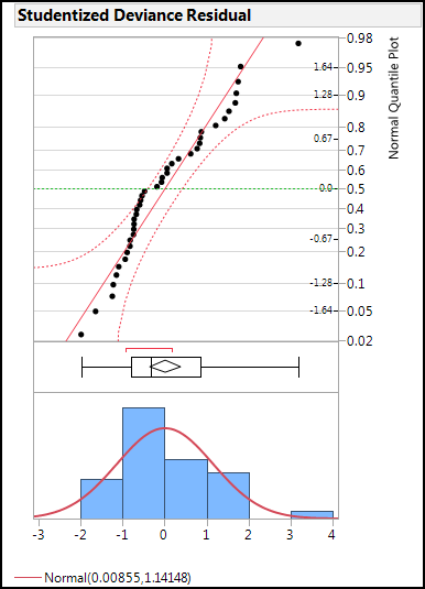
Returning to the question of the normality of the residuals, analyze the distribution of that column for normality with the Distribution platform (Figure 15.11). The normal quantile plot indicates the distribution to be normal enough for satisfying this assumption (most of the points are reasonably linear and fall within the 95% confidence limits of the plot).

Figure 15.10: Saving the Residuals

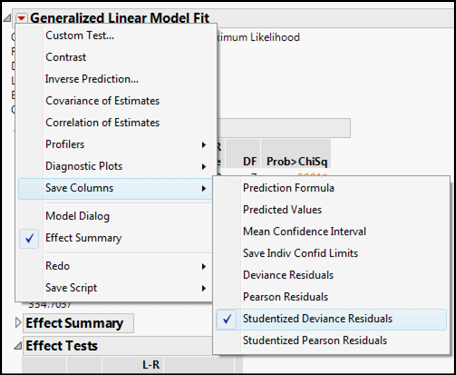
Figure 15.11: Residual Normality Evaluation

In this particular case, we can conclude that we are getting six of one and half a dozen of the other when comparing a standard least squares analysis to a general linear model approach. But we have made different assumptions for the two, and in cases where the data do not fit the assumptions of one, they might with the other, giving the analyst another tool in the toolbox. Generalized Linear Models are particularly helpful in the cases with a normal distribution is not expected, that is, the responses are binomial or count distributions.

Binomial Generalized Linear Models

The middle path on the generalized linear model flowchart (Figure 15.1) is used when the response to be modeled is binomial in nature. This model is also known as the binary logistic. And since we are going to be using the phrase “generalized linear model” a lot in the upcoming text, please note that this can be abbreviated with the acronym GLZM (in contrast to GLM for the general linear model of the last section).

Assumptions of the Binomial GLZM

This model does not assume that residuals are normally distributed or that the variance is homogeneous across the range of the explanatory variables. It is assumed that there is a linear relationship between the response variable that is transformed by the link function and the associated explanatory variables. However, this is difficult to assess, and in practice is usually ignored. Consequently, the residual plots have little value to the evaluation of the model.

The assumption that is easy to check since JMP can calculate it for you is the absence of overdispersion. As a reminder, overdispersion occurs when the variability in the data is larger than expected for the distribution used in the modeling. For the binomial and Poisson distributions, an overdispersion of about 1 is desired, and one considers it a violation of the assumption when the overdispersion exceeds a value of about 2. However, it has been noted that overdispersion is not uncommon in practice.8

How Severe Is It?

For an example problem, open the JMP sample data file entitled Liver Cancer.jmp in the provided sample data library. The first column tabulates the number of cancerous nodes found in the 136 subjects from which this data was measured. High severity is defined as > 5 nodes present. “Markers” refers to biochemical markers of liver function with a value of 1 indicating abnormal levels. “Hepatitis” refers to the presence (1) or absence (0) of anti-hepatitis B antigen antibodies, indicating infection with the hepatitis B virus. The jaundice column indicates the presence (1) or absence (0) of jaundice, which would also indicate a failure in liver function.

The biological question before us is whether any of the variables of BMI, age, time, markers, hepatitis, or jaundice can predict the probability of having a low or high node count. This would have diagnostic and prognostic implications if we could have some idea of the likelihood of the extent of the cancer spread given these variables that can be measured more readily than trying to find and count cancerous nodes.

To set up the analysis, open the Fit Model platform and transfer the Severity variable to the Y Role box and the BMI through the Jaundice variables into the Model Effects box. JMP assumes you want to do the Nominal Logistic analysis as soon as it sees a nominal variable as the Y variable, but we want to change that to the Generalized Linear Model (not to be confused with the Generalized Regression personality), as shown in Figure 15.12.

Figure 15.12: Setting Up a Binomial GLZM, Part 1

Once you have changed the Personality to Generalized Linear Model, choose the Binomial as the distribution. JMP will automatically assume you want the Logit link function, which we do in this case. Since a lack of overdispersion is an assumption for the binomial GLZM, check the Overdispersion Tests and Intervals box as well (Figure 15.13), and then click Run.

Figure 15.13: Setting Up a Binomial GLZM, Part 2

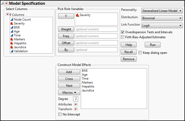
Figure 15.14 shows the most important output from this analysis after activating the Prediction Profiler using the Little Red Triangle for the Generalized Linear Model Fit.

Figure 15.14: Binomial GLZM Output

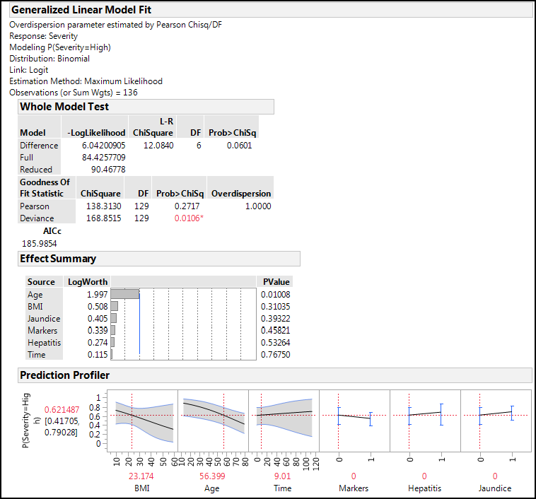
The Whole Model Test shows a p-value that is just above the statistical significance at the 0.05 level, but there is no overdispersion. (Remember, we expect a value of 1 and do not want to see anything above 2, if possible.) The Effect Summary shows that the Age variable contributes significantly to the probability of having a High Severity of cancerous nodes, but none of the other variables contribute significantly. Looking at the error ranges around the lines in the Prediction Profiler, we can see why: they are so wide we could drive a truck through them!9 The default values for BMI, Age, and Time are the averages of the data in each case, and we can read this to say that at these settings of parameters, we expect a 62% probability of having a High Severity, with a 95% confidence range of 42% to 79%. Again, this is a rather large range and a portion crosses the 50% line, meaning that the 95% confidence range encompasses both the Low and High Severity categories.

Since the Time variable has the largest p-value at 0.77, we can try eliminating it from the model to see whether that improves the outcome. Doing so reduces the whole model p-value to a significant value of 0.0348, leaves the overdispersion unaffected, and Age as the only significantly contributing factor. The predicted probabilities at the settings above remain unchanged as well. Looking at the AICc, it has dropped from 186 to 184, but that is a difference of less than ten, so it is not a practically significant drop.

In fact, given the high p-values for all but the Age variable, we can eliminate all but Age and still get a significant model (p = 0.0039) with no overdispersion. When doing so, the 95% confidence limit of the prediction at the average age now shrinks to 54% to 71%, a slight improvement.

Poisson Generalized Linear Models

The same data set we just evaluated provides an opportunity to also look at the Poisson GLZM. The first column contains the actual tumor node count used to divide the subjects into the two categories we just evaluated as a binomial distribution. But count data is a little different, remembering that we have only integer values in our distribution.

Poisson Distributions

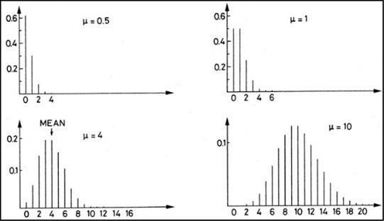
First, we need to recover our definition of the Poisson distribution from Chapter 4. This distribution is unique to count data. It consists of a discrete but continuous set of nonnegative integers only. It occurs when you are counting items that cannot be divided into subparts – in this case, tumor nodes. You either have one or you don’t. You don’t have half a node! Figure 15.15 shows some examples of Poisson distributions.

Figure 15.15: The Poisson Distribution

Counting Nodes

What we want to do now is see whether the same variables we previously examined in the binomial GLZM model can be used to predict the actual node count of the liver cancer. In setting this up, the only difference between what we entered in Figure 15.13 is that we have selected the Poisson Distribution under the Generalized Linear Model, and JMP has selected the Log Link Function for us (Figure 15.16).

Figure 15.16: Poisson GLZM Setup

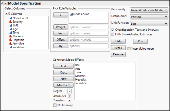
Figure 15.17 shows the output of this analysis.

Figure 15.17: Poisson GLZM Output

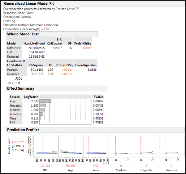
Again we have a statistically significant whole model, but this time our overdispersion is significantly different from the desired value, rendering our model of lesser utility. Looking at the Effect Summary, only Age is a statistically significant contributor to the node count. When we look at the Prediction Profiler, the responses do not show large effects, and the predicted node count is 5, with a 95% confidence range of 3 to 7, which is rather large for this context. Our overall conclusion might be that with this data, we are more likely to accurately predict the general severity of the cancer with the binomial analysis than we are to accurately predict the actual number of cancer nodes present. This might not sound exciting, but it is definitely helpful in the context of determining the prognosis of the patient.