Chapter 2: Thinking Statistically

“Poirot,” I said. “I have been thinking.”

“An admirable exercise my friend. Continue it.”

Agatha Christie, Peril at End House

Thinking Like a Statistician

Step One: What Is Your Objective?

Step Two: What Type of Data Do You Have?

Step Three (The Forgotten Step): Check Method Assumptions!

Summary

Thinking Like a Statistician

At the risk of sounding like we are about to embark on some mystical journey of introspection, the purpose of this chapter is set the stage for what is to follow. Here we want to consider how to think like a statistician. This is easier said than done, but is not an impossible task. Every discipline, whether it be some esoteric branch of mathematics or the more mundane field of car mechanics, uses its own thought processes in addressing the problems encountered in those fields. Statisticians are no different. They have concepts such as randomness, variability, error, probabilities, and averages to incorporate into their mental toolboxes as they consider the specific problems that they are asked to solve. Many of these concepts are relatively easy for beginners to master using the skills already acquired. But a few are more problematic, especially for those students desiring to apply statistical methods to their research but for whom the mastery of statistics is not their main goal. (As pointed out in the About this Book section, mastery of statistics is, alas, a necessary goal if not a main goal for a developing scientist.)

For example, as budding biological scientists, we might think the goal of an experiment should be to prove or disprove the hypothesis being tested by hopefully “proving” our hypothesis to be correct. Not so, says The Statistician. We can never “prove” a hypothesis, we can only “reject the null hypothesis.” The full rationale for this posture will be covered in chapter 6. For now, just note that this is a different way of thinking that will take some adjustment to our own thought processes as burgeoning scientists.

With that as an introduction, we want to consider in particular how to think like a statistician in selecting the statistical test that we are going to use on our data. What methods will we use to gather our clues to solve the mystery presented to us by our data? (Or, if you have a more warped frame of mind, you can think of it as how you will select the tools of torture to make the data scream out its story.)

This aspect of choosing the right test to use is probably the task that causes the most problems for beginning students. Practitioners of the art have, through experience, already worked this out so that it is second nature for them. Alas, the intended audience of this text lacks that experience (and often the desire) to attempt this with any confidence. To them I say, let not your heart be troubled. There is a method to the apparent madness, and it can be mastered. The process by which one determines what test to apply to one’s data is logical but requires the knowledge of some fundamentals of statistics, so even though we aren’t going to actually apply this process in practice until chapter 7, it will serve us well to cover this here in this chapter as it sets the stage for the intervening chapters.

Step One: What Is Your Objective?

This is the very first thing we must determine in this process. All too frequently the statistician is presented with a collection of data and asked to “analyze it” with no further elucidation of what the analysis is supposed to do. This is where the analyst must use his or her people skills to draw out exactly what the actual goal of the analysis is to be. Consider this famous interchange between Alice and the Cheshire cat:

“Would you tell me, please, which way I ought to go from here?”

“That depends a good deal on where you want to get to,” said the Cat.

“I don’t much care where— ” said Alice.

“Then it doesn’t matter which way you go,” said the Cat.1

But the goal really does matter, so to answer this question, we must know what statistics can do for us. What are the potential answers statistics allows us to find? Statisticians usually have two primary objectives:

1. Describe a population

2. Infer something from the data

Objective 1: Describe a Population

The first primary objective one can have is to simply describe a population. This is the process whereby we succinctly summarize a lot of numbers with a much smaller set of numbers that will allow us to visualize (at least to some extent) the data set that we are evaluating. We will cover this topic in detail in Chapter 4.

Objective 2: Infer Something from the Data

The second primary objective is to infer something from the data, and this forms the largest part of the arena of statistics. What does it mean “to infer?” Well, according to Webster’s Dictionary, and in this context, it means “to conclude or decide from something known or assumed; derive by reasoning; draw as a conclusion.”2 Basic statistical inference goals can be subgrouped by the specific goal, of which there are two.

One of the most frequent and clearest inference goals is to determine whether or not there is a quantitative difference between two or more samples that exceeds that expected by chance alone. Those samples may come when comparing samples of individuals or results from different methods. Chapters 9 and 10 will cover methods to achieve this goal.

The second basic inference goal involves determining whether or not there is an association or relationship between two or more variables in a set of data. If such a relationship exists, then additional goals include determining which variables are the most important and modeling the outcome or outcomes of interest using those variables (that is, predicting or forecasting results based on the models created). We will address these methods in Chapters 11 through 17.

Step Two: What Type of Data Do You Have?

There are three primary types of data the analyst will usually have to deal with, and each has its own methods for analysis. Consequently, JMP designates these types of data as “Modeling Types.” The three primary types of data are:

1. Nominal or categorical

2. Ordinal

3. Continuous

The first type of data is the nominal or categorical data type: variables that represent distinct units or groupings. The data itself can be either numeric or character, but the numeric will be code values for some grouping or category. Examples include variables such as gender, blood type, instrument, technician, and location. Each member of this type of variable is mutually exclusive from the other members of the variable grouping.

Cases that are categorical but have an order or sequence to them are called ordinal variables. Again, the so-called “raw data” may be collected as numeric or character values. However, there will be a sequence to them. For example, birth order is one such variable. Other examples would include such things as class in college, month, size (for example, small, medium, large), and letter grades. These share the challenges of categorical variables, but contain the additional information of order that requires slightly different treatment in doing the statistics.

Thirdly, there is the continuous data type, which is probably what most people will think of when they think of “data.” Continuous data is always numeric and its values are those with which we perform mathematical calculations such as addition or averaging. Examples include such variables as height, temperature, or time. Continuous data can be considered continuous in the sense that one can find an infinite number of values between any two values, that is, the range between two values can be continuously divided. Thus, we can have a value of 2.5 between 2 and 3, but if 2 and 3 are categorical labels of two instruments, you don’t have an instrument 2.5 between them.3

A distinct subclass of the continuous data type is present when the numbers represent counts of members of different categories. The counts are continuous but can only assume integer values of zero or greater. Such data is usually transformed into frequency data and analyzed as frequency distributions.

JMP identifies the modeling type of a variable by providing symbols alongside of the column names in the column summary to the left of the data table as shown in Figure 2.1.

Figure 2.1: Variable Modeling Type Symbols

What test is to be chosen to analyze the data will depend on the data type (modeling type).

Also to be considered here is how the data was collected – that is, the experimental design. We will be examining some of these issues in the next chapter (Chapter 3). In Chapter 9, we will see that collecting the data in a paired manner can have a significant effect on the outcome of the analysis. Meaningful data analysis requires some knowledge of experimental design, and, indeed, that experimental design can make or break the attempted analysis, so it is necessary to consider what type of data analysis you want to do as you design the experiment in the first place.

Step Three (The Forgotten Step): Check Method Assumptions!

This is the step that I have personally observed is all too frequently not done. The primary question the analyst needs to ask is, do the data match the underlying assumptions of any given analysis method closely enough to permit the valid use of that analysis method? Failure to check assumptions can lead to the generation of a lot of meaningless numbers. The software can calculate the statistics and give you p-values upon which to ruminate, but if the assumptions of the test used have been violated, the results are worthless at best and misleading at worst.

As just one example, parametric tests assume some aspect of the data is sampled from a normal distribution. JMP (and most statistical software applications) will give you the results of a parametric analysis even when this assumption is not true. Reliance upon the software is not to be done blindly. We must assert with Hercules Poirot, “These little grey cells. It is up to them.”

Summary

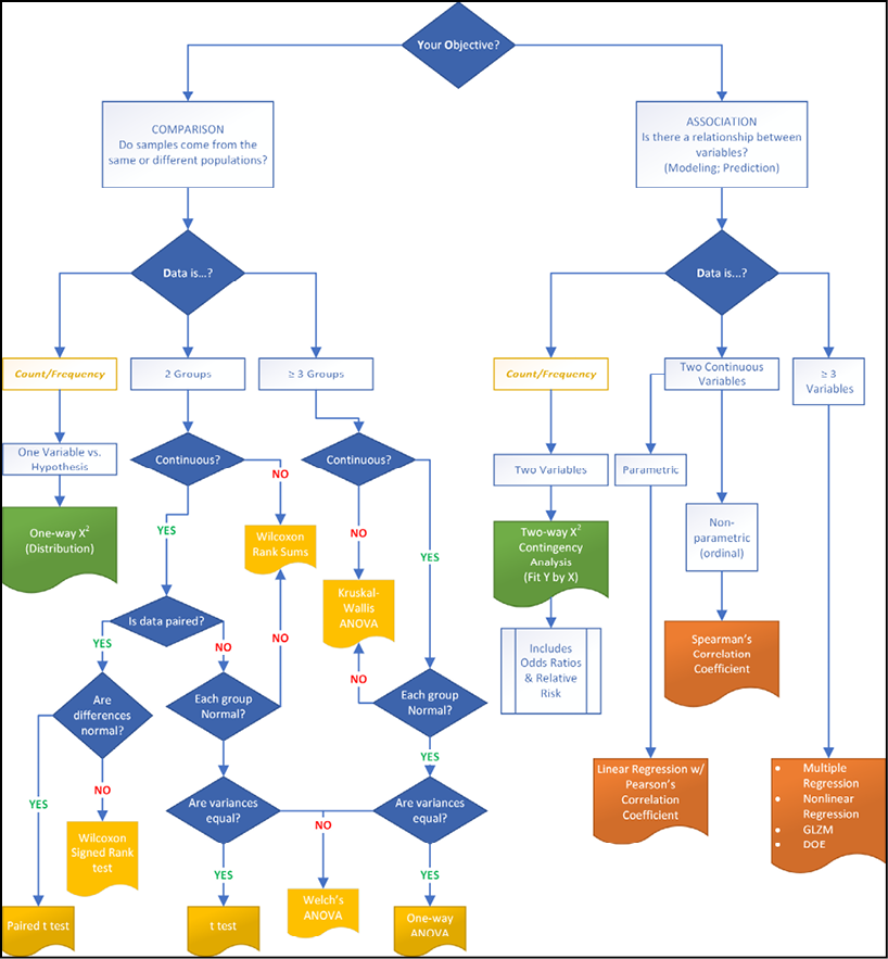
The observant reader will have noticed the italicized and underlined letters in the titles for the steps in this chapter, which give us a memory device to be able to recall these three steps: Y.O.D.A. Throughout the rest of this book, any reference to the Y.O.D.A. strategy will be pointing you to this simple set of steps for statistical thinking on which to base your analysis. In fact, once we cover the preliminaries, the rest of the book will proceed with this logical process and is outlined in a flowchart in Figure 2.2 below. This flowchart allows the student to determine what test to use with the Y.O.D.A. strategy.

Figure 2.2: Test Selection with Y.O.D.A. Strategy