Chapter 16: Design of Experiments (DOE)

All models are wrong, some are useful.

George Box

Introduction

What Is DOE?

The Goals of DOE

But Why DOE?

DOE Flow in JMP

Modeling the Data

The Practical Steps for a DOE

Step 1: State and Document Your Objective

Step 2: Select the Variables, Factors, and Models to Support the Objective

Step 3: Create a Design to Support the Model

Step 4: Collect the Data Based on the Design

Step 5: Execute the Analysis with the Software

Step 6: Verify the Model with Checkpoints

Step 7: Report and Document Your Entire Experiment

A DOE Example Start to Finish in JMP

Introduction

In this chapter we will attempt to introduce a topic about which volumes have been written by people much smarter than this author. But it is an incredibly powerful tool that every scientist should have in his/her toolbox. There is a multiplicity of books out there, including many available by and from SAS. Here we will only scratch the surface of this methodology1, but hopefully this will serve to whet the reader’s appetite to both appreciate and master this technique in the early course of their career so as to reap the benefits thereof. So…off we go!

What Is DOE?

Perhaps the best way to approach answering this question is to first say what it is not. First of all, it is not what we see in Figure 16.1.

Figure 16.1: One Thing DOE Is Not!

And it is likewise not:

Figure 16.2: Another Thing DOE Is Not!

So enough already with the silliness and just tell us what DOE is! DOE in this context stands for Design of Experiments. Now, astute readers, or at least the ones who are still awake, should immediately have a question jump into their minds: But wait! Aren’t all experiments “designed!?” What makes this so special it gets a whole chapter in this book?

Well, I’m so glad you asked that question! Yes, it is true that all experiments, at least all good experiments, have a significant planning component to them that is a design process. However, not all are designed with the end analysis in mind, and not all meet the primary requirement of a DOE. To the first point, many experiments get designed and executed, and then the data is taken to a data scientist who is then asked/told to “analyze this” for us please. Sometimes that works, but more often, not. A good design process also includes thinking about how you are going to analyze the data after you have collected it so that you can ensure you are collecting the right data in the first place, and that you can, indeed, get something out of the use of the time and resources the experiment will consume.

To the second point, what is the primary requirement of a DOE? The primary requirement of a DOE is the ability to vary all the important input parameters to the desired levels. Many types of experiments do not allow you to set the inputs of the situation; rather, you can only observe the inputs and record them accordingly. For example, if you want to determine how the amount of actual sunlight (using the actual sun) affects plant growth, you cannot turn a knob on the sun to adjust the lumens to specific levels at specific times; you can only determine how much is reaching the plants as a function of time. We cannot control the many factors that would influence the extent to which sunlight reaches the ground.

So what would be a helpful definition of DOE for our purposes? In his book Design and Analysis of Experiments, Douglas Montgomery describes it as “the process of planning the experiment so that the appropriate data that can be analyzed by statistical methods will be collected, resulting in valid and objective conclusions.”2 Mark Anderson and Patrick Whitcomb characterize it as “a planned approach for determining cause and effect relationships.”3 A third set of authors indicates that DOE “consists of purposeful changes of the inputs (factors) to a process in order to observe the corresponding changes in the outputs (responses).”4 (Emphases added.) Notice that the italicized portions of the preceding descriptions all align with the idea of planning out, of designing, very specifically the nature of the experiments to be executed. Combining the several ideas contained in these characterizations, the following definition has been derived by Yours Truly:

DOE: the generation of response data from systematically selected combinations of input factors that are used to create mathematical models (equations) from which valid and objective conclusions about the inputs and outputs can be inferred.

In addition to the idea of design, this definition introduces the concept of modeling and the ultimate goals of DOE.

The Goals of DOE

There are two primary types of DOE, each with their own primary goal. The first goal is simply to identify the important factors that contribute to a given response. The DOE design type with this goal is called screening, and screening designs typically allow for many factors to be evaluated but not necessarily with enough data collected to create a mathematical model that can be used for prediction. (Remember, as observed by that eminent statistician, Yogi Berra, “Prediction is very hard, especially when it is about the future.”)

Consequently, the second possible primary goal would be to predict a response based on the input variables that are the principal drivers of that response. This type of design is called a Response Surface Model (RSM) and collects more data with fewer input variables to gather enough information to be able to create a mathematical model of the process under evaluation. We will look at these two in more detail shortly (in other words, don’t stop reading here…unless, of course, your house is burning down around you).

Although the previous paragraphs outline the types and goals of DOE in neat categories, it should be noted that Mother Nature does not always play by these rules. That is to say, sometimes she has processes that are simple enough that a screening design can, in fact, be used to accurately predict outcomes as well as identify the major players, rendering a further RSM unnecessary. In addition, more recent work has developed a newer version of the screening methodology called a Definitive Screening Design5 that is even more likely to allow for both screening and prediction. And, of course, one can create, execute, and analyze these in JMP, although these are beyond the scope of this text.

A secondary, but equally important, goal underlying DOE is the idea of getting your results by consuming a minimum of your available resources. As we shall see, trying to measure all possible combinations of our input variables in a set of experiments can quickly lead to impossible numbers, whereas DOE can achieve statistically confident results with much fewer runs, as long as one designs those runs from the outset using DOE methodology.

But Why DOE?

Perhaps the best way to answer this question is by way of contrast to OFAT. This is, of course, another acronym, this time for One Factor At a Time, the time honored, traditional (and, indeed, correct) way of doing most experiments by the scientific method. The experimenter tries to design the experiment such that the only thing changing is the putative cause of the effect of interest, controlling by holding constant as many other potential variables as possible. In most cases, this is the best approach. But in characterization experiments, when one is trying to determine the factors that most influence a response of interest, or when one wants to be able to predict a response of interest based on critical input variables (think a manufacturing process here as a concrete example), OFAT has three basic flaws:

1. It can miss the true optimum settings of your input variables

2. It does not account for possible interactions between the input variables

3. It has a lower statistical power of analysis (when running the same number of experimental runs) than does a DOE approach

I have to take the statisticians’ word on number 36, and we will discuss interactions a little later in this chapter. To illustrate the first problem, consider the response in Figure 16.3 that is a function of input X and input Z.

Figure 16.3: An OFAT Example

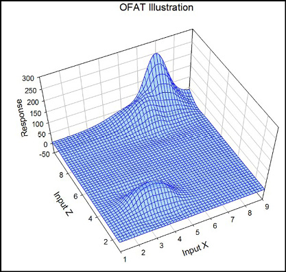
The optimum response (assuming we are looking to maximize said response) is clearly at a value of Z = 10 and X = 7. But there is a suboptimal maximum also at Z = 4 and X = 3.8. If the investigator fixes Z somewhere around a value of 4 and then tests various levels of X, that suboptimal maximum is what will be ultimately identified as the maximum, when, in fact, it most certainly is not. DOE systematically probes the entire surface as part of the design process, which makes it much more likely you will find the true optimum response. And it can do it when more than two variables are critical to your response, something graphing responses as we did above cannot do.

DOE Flow in JMP

There is a logical flow to DOE in JMP, and it is illustrated in Figure 16.4.

Figure 16.4: The Logic of DOE in JMP

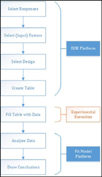
JMP provides an entire DOE platform, and the first four steps are carried out in that platform. There, you first select the responses of interest, and there can be more than one (and yes, you can use JMP to simultaneously optimize, if it is at all possible, two or more responses). You then input the factors that you want to investigate and their levels (more details about the mechanics are found later in this chapter). You select the design that you want to use to collect your data. Design selection refers to determining what combinations of factor to run. Figure 16.5 illustrates some of the classic designs for three variables with low, medium and high settings for inputs.

Figure 16.5: Classic DOE Designs

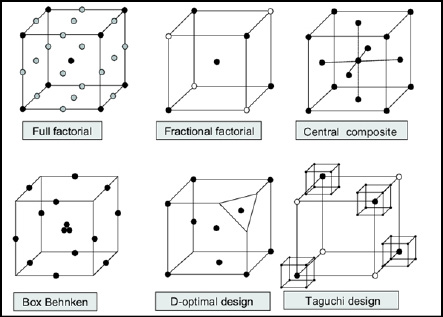
The full factorial design in the upper left of Figure 16.5 tests every possible combination at all three levels of each variable, and you can readily see how many tests need to be made (those would be the dots in the illustration). The other designs will allow for the same conclusions to be drawn with the use of much fewer resources thanks to the wonders of statistical math!

Finally, have JMP create a table that specifies the exact input variable setting combinations you will then run into the lab/factory/location of your choice to fill with real numbers (your data).

This is the point where you go have fun collecting your data to fill out the table JMP has provided. (And if this is not a fun part your work, you might want to reconsider your career plans.)

Once you have your data, you return to JMP for the “really fun” fun to begin, because now we are going to try to find out what story your data is trying to tell you. (Was it the butler in the kitchen with the candlestick?!) But we should now be in familiar territory, because all we are doing at this point is modeling the data with the Fit Model platform that we have been using since Chapter 13. Modeling in this context is simply creating the equation that connects the input variable(s) to the response variable(s) with all the diagnostic outputs that tell us how important each variable is to the response and how well our model fits the data.

Modeling the Data

To more fully grasp what we mean by modeling (no, we are not making model planes, or showing off the latest fashion!), consider a response y as a function of two input variables (because that is the easiest and clearest to visualize graphically) x and z. What modeling does is create equations that describe response y in quantitative terms of x and z. But what might that look like?

The simplest model is a linear model in which there is a slope in the x direction but none in the z direction (Figure 16.6).

Figure 16.6: A Linear Model Graphed

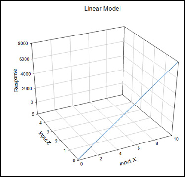
The equation for this model is the well-known y = a + bx, where a is the y intercept and b is the slope. In modeling, the statistics are calculating the best a and b, called coefficients, that create the best line that fits the data. (See Chapter 11 on linear regression.) This identical process is what is going on behind the curtains with the math for more complex equations as well.

The next most complex model would be a simple plane (Figure 16.7).

Figure 16.7: A Planar Model Graphed

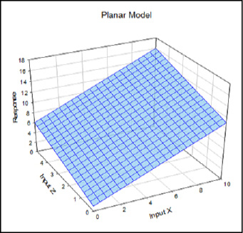
Now we are looking at the equation, y = a + bx + cz, where x and z are called “main effects” because they stand alone without interacting or being squared or being otherwise subjected to any additional mathematical manipulations. The model accounts for no interactions between the input variables, or for any curvature in the response surface. Because of its simplicity, it is often used to analyze screening designs where the primary goal is just to identify the major players contributing to a response.

So what does adding an interaction between x and z look like? I’m glad you asked! Figure 16.8 shows that the interaction term, expressed mathematically as dxz, twists the plane without adding curvature to it (yes, I know it looks like it does, but that is an optical illusion, I assure you; place a straightedge on any of the lines and you will see they are all straight with no curves):

Figure 16.8: An Interaction Model Graphed

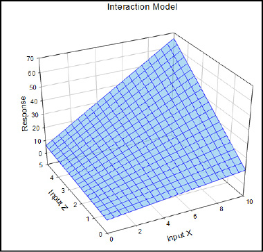
Our equation has now grown to y = a + bx + cz + dxz, where the xz is the interaction term.

How do we add curvature to the response? This is achieved with squared terms. Figure 16.9 shows what it looks like to add curvature in the x variable only.

Figure 16.9: A Curve in X Graphed

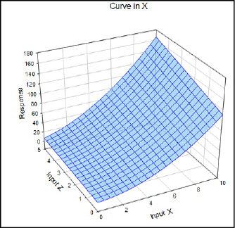
As we add each feature to our potential response, our equation to describe the response gets more complex. Now it looks like: y = a + bx + cz + dxz + ex2.

The quadratic equation allows for curvature in all variables, and we add the z squared term to our expanding equation: y = a + bx + cz + dxz + ex2 + fz2. See Figure 16.10.

Figure 16.10: A Quadratic Model Graphed

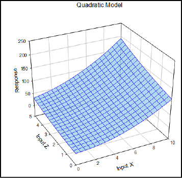
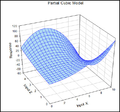
The quadratic model is most frequently used to analyze standard response surface designs. Fortunately, the overwhelming majority of cases you are likely to encounter in the biological world do not get more complex than this. For those that do so, there is the partial cubic model that allows for curves both up and down in all variables. The “partial” label is due to the absence of the actual cubed terms in the equation. The equation for a partial cubic model is y = a + bx + cz + dxz + ex2 +fz2 + gx2z + hxz2 (Figure 16.11).

Figure 16.11: A Partial Cubic Model Graphed

The Practical Steps for a DOE

So much for the theory, which provides much of the “why” of what we do when executing a DOE. Let’s turn our attention now to practical principles of execution. Figure 16.4 outlined the three major phases of DOE, but each one consists of several steps that can also be identified. In fact, we can distinguish seven steps from start to finish.

Step 1: State and Document Your Objective

If you aim for nothing, you are bound to hit it. Are we interested just in identifying the major players of a process, or do we really want the ability to predict our response(s) so that we can optimize our outputs? The former would only require a screening design in which more factors can be evaluated with a simpler response surface. The latter, however, is a response surface design that requires fewer variables to be involved so enough data can be collected to model a potentially more complex surface. If your process has never been characterized before, how many variables do you have to evaluate? Will you need a screening experiment first to weed out the inconsequential variables before setting up a response surface experiment? As you consider the options and your particular case, it would be well to remember J. W. Tukey’s admonition that “It’s better to solve the right problem approximately than to solve the wrong problem exactly.” It’s also a good idea to write down your objective both to communicate it to others and to remind yourself as you proceed just what it is you are trying to accomplish.

Step 2: Select the Variables, Factors, and Models to Support the Objective

Selecting Variables

This is where the JMP DOE Platform comes into its own. JMP first asks you what response or responses (the dependent variables of your experiment, the “y’s” of your equation) you want to model, and then what factors (the independent variables, the “x’s” of your equation) you want to use in that modeling. If you are in a biotech or industrial setting, the responses are the critical quality attributes your product needs for the customer to be willing to buy it. In a more research-oriented setting, the responses are the things of biological interest and importance that you are investigating.

The variables that we will consider here are continuous and categorical variables, but one can also model mixtures and use blocking variables. These latter two considerations, while important, are not within the scope of this introduction to biostatistics, but you should be aware that they exist.

The selection of the responses and factors is perhaps one of the first places that the “art” of science enters the picture. This process requires a good knowledge of the system that you are investigating, and there are no hard and fast rules that can be given for how to select the right ones. Preliminary experiments can be helpful, especially when setting the ranges for your independent variables. But the bottom line is, you need to know the biology and/or the chemistry of your system to be able to make intelligent choices.

In addition to the variables that you want to investigate, this is probably the point at which you should also consider potential noise variables and identify those variables that you want to control at constant settings for your system. There will almost always be potential inputs that are not of interest to the study and, if at all possible, should be set to a fixed control level for the duration of the experiment. There are likewise potential inputs that cannot be controlled and could influence results and should be monitored (that is, recorded) so that, if necessary, they can be evaluated as random factors to see whether they have influenced your response. Examples of such noise factors include things like ambient temperature and humidity.

Setting Ranges

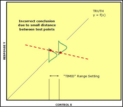
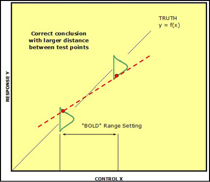
A word about setting the ranges of your variables for the experiments that you are about to execute. This is particularly important for the continuous variables. You will want your low and high settings to be far enough apart that you will maximize your chances of seeing a difference that you can model. But it is important to also remember that there is going to be some level of measurement error. This being the case, if the range is set too “timidly,” that is, too close together, there is an increased possibility that the measurement taken at the low setting might be on the higher part of the response curve, the measurement at the high setting might be at the lower end of the response curve, and the subsequent conclusion drawn could be the exact opposite of the real response (Figure 16.12).

Figure 16.12: “Timid” Range Setting...Bad

By selecting the low and high range settings farther apart (that is, “boldly”), this error can be avoided even when the same measurement error combination is encountered (Figure 16.13).

Figure 16.13: “Bold” Range Setting...Good!

What Model?

Once the factors have been chosen and the responses selected, the next question is, how do you want to have the x’s related to the y’s? In other words, what equation do you want to evaluate as a potential model for your responses? Do you want to look at main effects only, or do you want to include the potential for interactions and evaluate those? Here is where your experimental goal integrates with your decision because a screening design will most likely only look at main effects, but include many more independent variables. For a response surface design, you generally have fewer variables (3–4 at maximum) and can afford to look at more complex models that take into account interactions and curvature.

Since the data collected to support a complex model will also support less complex models, a commonsense approach is to try to create the most complex model you can under the specific conditions of resources that you have available. This then leads us to step 3.

Step 3: Create a Design to Support the Model

At this point we are now ready to select the combinations of variable settings for which we will collect data to use in constructing our mathematical model of the phenomenon under study. Rather than worrying about figuring out these combinations ourselves manually, the JMP DOE platform will do all the heavy lifting for us at this point. The only designs we will look at in detail here are the optimal designs selected by the Custom Design platform. This generally provides the most flexible of design choices for most purposes. However, it should be noted that JMP has the option to choose many other designs as shown in Figure 16.14.

Figure 16.14: Other Design Options in the DOE Platform

You can see that, in addition to the Custom Design option, you can select Definitive Screening designs, classical screening and response surface designs. If you are a glutton for punishment and have unlimited resources, you can choose a full factorial design, and if you need it, you can do mixture designs. If you are in marketing, you might be interested in the choice designs found in the Consumer Studies menu shown above. All of these have their place in the toolbox of the researcher, but are beyond the scope of this present work. I call your attention to them to hopefully whet your appetite for this rich menu of powerful tools provided in this platform.

Replication

As we turn our attention now to design, there are a few considerations that we should note. JMP will ask whether you want any centerpoints and replicates. Centerpoints will be points in the middle of the response surface plane that can help detect curvature if they are used. Replicates are used to help measure process error, but be forewarned that a replicate to JMP means a complete new set of runs based on the initial design. Thus, if the initial design calls for 8 unique combinations, one replicate will generate a design with 16 runs, the unique 8 combinations created twice.

True replication is repeating all the steps of the process under investigation so that each set of conditions is executed as a unique run more than once, starting from the beginning. This allows the underlying math to calculate the process error associated with your model, taking into account the variation of the system and ability to reproduce the phenomenon in question. This is to be distinguished from measuring the response from the same preparation multiple times, which quantitates the measurement error, not the process error. Some sources would call this type of replication pseudo-replication since you are not evaluating the entire process. That prefix “pseudo” carries some negative connotations that make it sound like a bad thing. This is only true if the investigator is not aware of what he or she is truly measuring. There are times it is quite important to know the amount of error is being introduced into the results by the instrument measuring those results, that is, the measurement error as well as the process error.

Blocking

There will be times when factors will be identified that are not of interest to the problem under investigation but which might still impact the results. For example, you are interested in determining whether a dog’s running speed is impacted by its diet, and you have four different diets to test and a population of 100 dogs (of the same breed) to work with. A variable that could affect speed is age, yet you are not really interested in the effect of age on speed, but the population of dogs available for the study are of different ages. While you could randomly assign the dogs to each diet group and hope your ages are spread evenly across your four groups, a better approach is to treat age as a blocking factor in the experiment. To do this, you would rank the dogs by age and then partition the ranks into blocks so that those in a given block have a similar age. The number of blocks is not of great importance to the analysis, only to the logistics of the execution. What is important is that the number of subjects in a block is a multiple of the number of test groups. (In this case, we have four diets, so we need multiples of four in each block.) The subjects in each block then get randomly assigned to the test groups so that now each test group has approximately the same type of population relative to the variable being blocked (in this case, age). Treating the blocked variable as a separate factor in the data analysis allows you to determine whether, in fact, this variable has influenced your results, and, if so, to remove its influence from the analysis of the remaining factors.

If all that sounds complicated, it is. But rejoice! JMP will handle all that planning if you simply identify age as a blocking variable when you set up the experiment in the DOE platform. It will then separate out the individuals from each block into their appropriate groups for you. Software is so much fun!

Confounding and Aliasing

In a DOE experiment, more than one variable is usually being changed at a time. Therefore, another concern when selecting a design is what happens when two different alterations are applied to the same process at the same time so that if the process response changes, you do not know which alteration caused the change. For example, you get stung by a bumblebee on your finger as you reach for a flower. Having avenged itself upon your poor finger, the bumblebee flies off, leaving you behind doing the not-so-happy bee sting dance with accompanying vocalizations unfit for print. Someone eventually grabs you, after downloading your dance choreography to Facebook, plants you in a chair, and sticks your throbbing hand into a cold glass of ice water, whereupon you sigh the sweet sigh of relief as the pain subsides and you can now think rationally enough to threaten with bodily harm whomever did download this episode to Facebook. Question: what relieved the pain, the wet of the water or the cold of the ice? We don’t know, because “wet” and “cold” are confounded or aliased.

Statisticians have “repurposed” the concept of resolution from microscopy to address this and to signal how the variables of a DOE might be confounded with one another.

● Resolution-3 designs: main effects not confounded with each other but are confounded with 2-factor interactions; only main effects are included in the model.

● Resolution-4 designs: main effects are not confounded with main effects or 2-factor interactions, but some 2-factor interactions are confounded with each other.

● Resolution-5 designs: no confounding between or within main effects and 2-factor interactions.

Since the best situation would appear to be to always choose resolution-5 designs, why bother with lower resolution designs at all? Simply for the pragmatic reason that increasing the design resolution increases the number of trials needed to get enough data to make the distinctions needed to separate out confounded variables. This, of course, means using up more resources, and such resources might be limited to the point that resolution-5 designs may not be possible under the conditions available. Thus, the only two choices would be to weep, wail, and gnash one’s teeth, which really does not help much, or to run a lower-resolution design to get at least some information that can be applied to solving the situation at hand.

New(er) Designs

Back in Figure 16.14, we noted that JMP includes the ability to create so-called classic designs through the DOE platform. Some of those are diagrammed out in Figure 16.5. The Custom Design menu focuses on designs that have been created in the more recent history of DOE as improvements on the classical designs (not that the classical designs are misleading or incorrect), the “optimal” designs.

If you have a fairly large number of variables, you will most likely find JMP creating a D-optimal design for you. This design seeks to maximize a criterion so that you learn more about the variables themselves. For those who really want to know, that criterion minimizes the generalized variance of the estimates. (And no, I don’t really know the math behind that statement, but as biological scientists, we only need to know that it is valid and it works, with apologies to my mathematical/statistical friends.) It is an all-purpose design particularly useful for screening designs.

In other situations, you will find JMP creating an I-optimal design. This design maximizes a criterion so that the model predicts best over the region of interest and has the most utility in response surface optimizations. (The criterion cited minimizes the average variance of prediction over the experimental region.)

A Final Design Point

When you come to the point of having JMP create your data table that you will take into the lab for data collection, the default option is to randomize the trials, but there is the ability to change that to other, more orderly sequences. Unless there is a compelling reason to do otherwise, randomization is the best choice to reduce correlations between the independent variables of the study and unknown confounding variables. As R. A. Fisher noted, “Designing an experiment is like gambling with the devil. Only a random strategy can defeat all his betting systems.”

Step 4: Collect the Data Based on the Design

Once you have your JMP data table without data, you get to have the real fun that you have been looking forward to all along: doing the actual experiments and/or making the observations that started you on this journey in the first place. On a historical note, much of the original development of DOE methodology came from the agricultural field (or fields, literally) and the beer brewing industry, so the techniques have their roots (pun not intended) in biology.

There is a possibility that you will not be the one collecting the data personally, or that you will be working in a team and that someone else will be helping collect the data. It may be that you need to have samples run on a certain instrument that you are not qualified to use, so a trained technician will be running the samples for you. Regardless, get involved as much as possible with the data collection. “There is nothing like first-hand evidence,” as noted by that eminent statistician, Sherlock Holmes.7

If others are involved, share the ownership of the project; communicate why and how you are doing things. I don’t know how true they are, but I have heard anecdotes of how someone planned out an experiment and did not do this, and the “old hands” in the factory who just “knew” how things would turn out, filled in his data table with numbers that they just “knew” would be the outcomes without actually doing the actual process at the requested settings, and their knowledge was not accurate despite their experience. As you might imagine, the results were less than satisfactory.

Step 5: Execute the Analysis with the Software

For those of us diagnosed with clinical insanity due to our love of statistics, this is where our fun really gets fun! You now have your data table filled out with real data from your efforts, but what does it all mean? We are done with the DOE platform at this point and move to our old friend, the Fit Model platform. Analysis in this context simply means combining your data with math to create an equation of your process. In doing so, we want to answer two main questions: does the model fit the data, and what are the important factors and variables? Table 16.1 summarizes some of the metrics provided by JMP that allow the analyst to answer these questions. Notice that we generally do not have to rely upon just one value to make a decision.

If we are in a screening design, the answer to the second question furnishes us with the information for the construction of a response surface DOE. If they are already from a response surface experiment, then those are the variable for the axes of the contour plot and the focus of our attention in the Prediction Profiler.

Table 16.1: Metrics Provided by JMP to Assess DOE goals

Metric	Model Fit	Important Factors	Comments
RSquare	X		% of variation in the response data accounted for by factors in the model
RSquareAdj	X		Adjusts the RSquare value to make it more comparable over models with different numbers of parameters using the degrees of freedom to penalize those having many model terms
p-value, whole model	X
AICc, BIC	X
p-value, LOF	X
p-value, individual factors		X
Normal plot		X	Significant factors appear as outliers that lie away from the line that represents normal noise (and helpfully labeled for you by JMP)
Prediction Profiler	X	X	95% confidence limits of prediction and error bars provided when possible to calculate help in assess model fit and important factors

Step 6: Verify the Model with Checkpoints

Remember the quotation from George Box at the beginning of this chapter: “All models are wrong, some are useful.” At this point, you have a model and presumably it has a reasonable fit to the data, at least the data that you used to create it. Checkpoints or verification points are trials run at combinations of settings not used to create the model, or, in other words, predictions that will hopefully prove that your model has some contact with reality. This is a vital step if the model is to have demonstrated utility beyond working only on the data use to create it, which would amount to arguing in a circle. At what settings should you try to create checkpoints? Several options are available to you, including at or near optimum response outputs, near suspicious behavior, at low cost settings, and even at settings outside the range of the original settings (how well does the model extrapolate?). But regardless of where, one should always, always, always (did I say that often enough?) check the model’s predictions to verify whether it has utility beyond the settings used to create it.

Step 7: Report and Document Your Entire Experiment

Information is useless unless shared. One would think it unnecessary to state this as bluntly as this, but it is. I spent 25 years of my life in an industry where if you did not document it, including signing, dating, and having it signed and dated by a witness, it never happened. Period. Your documentation requirements might not be as stringent, but it is better to be safe than sorry.

In addition, this documentation should really go beyond a simple “here is what I did” approach frequently found in lab notebooks. Particularly with DOE, document the logic and rationale of all your steps (for example, why did you choose this range for this variable?) even if it seems obvious to you at the time. It will help tremendously when you have to defend it to your doctoral review committee, or your friendly neighborhood regulatory agency (for example, the FDA) three years later when you have forgotten all those little details that are currently seared into your consciousness and you think you could never possibly ever forget.8 Trust me, you will. It is best to remember what Confucius says: “The weakest ink is mightier than the strongest memory.”

A DOE Example Start to Finish in JMP

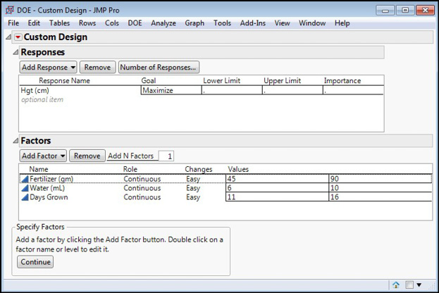
Since agriculture was one of the first places in which DOE methodology was developed, we are going to try to maximize plant growth by modeling said growth on three factors: amount of fertilizer, the amount of water, and the numbers of days the plants are allowed to grow. We will see how successful we are modeling with just two levels of each (Table 16.2).

Table 16.2: DOE Domain Ranges

Factor	Low	High
Fertilizer	45 gm	90 gm
Water	6 mL	10 mL
Days grown	11 days	16 days

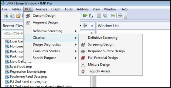
Open the Custom Design DOE dialog box and enter the information shown in Figure 16.15 (DOE / Custom Design).

Figure 16.15: Custom Design Dialog-Response and Factors Entered

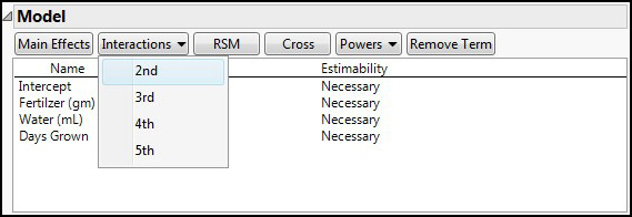
Clicking Continue takes us to the next step, determining the model that we want to try to construct. We know we want to include the three variables as main effects, which JMP defaults to adding to the model. Given the possibility of interactions between the variables, we should also add two-way interactions by selecting 2nd under the Interactions drop box for Model to add these to the desired model (Figure 16.16).

Figure 16.16: Adding Interactions to the Model

The default number of runs with these parameters is 12, but given the ease of getting the supplies for this experiment, let’s add four more runs by entering 16 into the User Specified box, and then clicking the Make Design button (Figure 16.17).

Figure 16.17: Adding Runs and Making Design

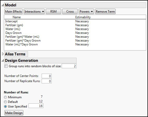
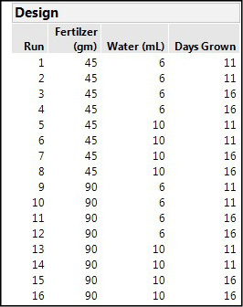
Normally the design that JMP creates and displays is randomized, but the Design in Figure 16.18 has been ordered Left to Right to see that we have eight unique runs, each duplicated. Had we used the default of 12 runs, four runs would not have been duplicated, and we will see shortly the impact that adding just those four runs has on the overall model efficiency.

Figure 16.18: The Design Created by JMP

Having created the design, JMP provides several ways to evaluate the design under the Design Evaluation node. Probably the most useful are the Color Map on Correlations, which enables you to see which variables are aliased and to what extent, and the Design Diagnostics, which gives some efficiency metrics of the design (Figure 16.19).

Figure 16.19: Some Design Evaluations

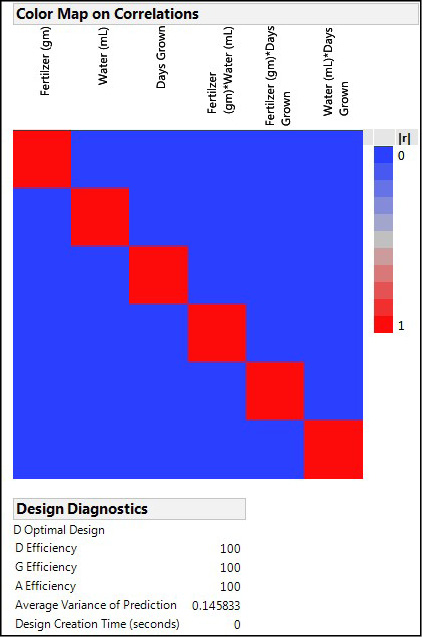
The color map will show aliased variables with correlations greater than zero, which is really not what we want when at all possible. The diagonal line of red boxes is simply the variables correlated to themselves, which we would hope they would be. This color map is the optimal one we want to see, where none of the variables, be they main effects or interactions, are aliased with any other variable.

The Design Diagnostics calculate the various efficiency metrics, and we would prefer to have 100% efficiencies, which is what we do have with this design and this number of reps. JMP also tells us it has created a D optimal design for this set of variables and this number of levels.

Now, click the Back button at the bottom of the window and select the default number of runs of 12 for your design, and make that design. The same design evaluation nodes now show you that merely reducing the number of replicates of those unique runs by 4 out of the eight has introduced some aliasing as well as reducing the efficiency of the design (Figure 16.20).

Figure 16.20: A Less Efficient Design by Comparison

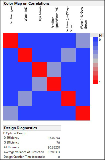
Notice that now the Fertilizer main effect is aliased with the interaction between water and days grown with a correlation of about 0.5 as indicated by the gray colored squares where those two variables intersect in this graphic. In fact, each main effect is aliased with a different two-way interaction in this design.

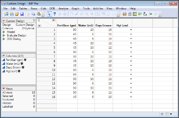
Go Back again and restore the full 16 runs, make the first design again, and then click the Make Table to create the data table without data that you are to take into the lab (or greenhouse in this case) to grow some plants under these specific combinations of fertilizer, water, and number of growth days (Figure 16.21).

Figure 16.21: The Data Table to Be Filled Out

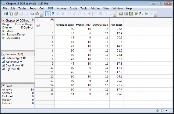
In this case, we do have data that has been collected and is shown in the next figure (Figure 16.22).

Figure 16.22: The Data Table Filled Out with Data

We are now ready to have some analytical fun by seeking to model the data in the Fit Model platform. We can set this up using either the script JMP has created by clicking on the little green triangle in the script box on the top left side of the data table, or by simply opening the Fit Model platform through the standard menu. Either way will result in the model specified in the DOE setup being entered for the analyst into Y variable and model effects boxes, complete with the interactions that we want to include in the model (Figure 16.23).

Figure 16.23: Fitting the Model with the Fit Model Platform

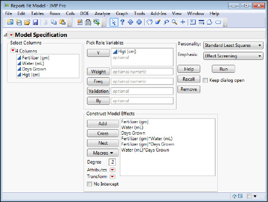
When there is any chance I might want to evaluate more than one model, I personally find it helpful to check the Keep dialog open box so that I can redo the analysis by rearranging the model effects. For now, let’s leave all the main effects and two-way interactions in the model and see what we get. Click Run and you should get the analysis that we will now look at in detail in the next several figures.

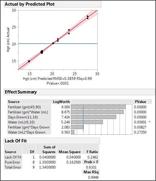
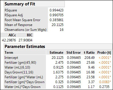
Figure 16.24 shows us that we have a very good model in this case. The RSquare value indicates we are accounting for 99% of the variation in the height with our model, and there is no significant lack of fit (p = 0.6331). All but one interaction is contributing significantly to the model. The Effect Summary node ranks the variables by their logworth values, which gives a quantitative estimate of how much each variable is contributing to the response. This is particularly useful when the p-values are all so low that JMP just assigns them a value of < 0.0001. So the variable contributing the most to the plant height is the amount of fertilizer, followed by the interaction of the fertilizer and water.

Figure 16.24: Analysis, All Variables Present, Part 1

The remaining output of interest (Figure 16.25) confirms the very strong RSquare values, gives values for AICc and BIC for comparisons (we will compare the main effects only model in a moment), and the parameter estimates. Those parameters (the coefficients in the equation) are all positive, indicating that the height increases in direct proportion as the values for these variables increase.

Figure 16.25: Analysis, All Variables Present, Part 2

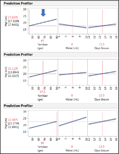
The strongest interaction (Fertilizer * Water) is evident in the Prediction Profiler when we leave the water and days grown at their midpoints (the default values JMP uses when the Prediction Profiler is first accessed) and move the amount of Fertilizer used from the low to midpoint to high amount of fertilizer (note the arrow in Figure 16.26 and the vertical dotted line). The slope for the amount of Water goes from positive at high Fertilizer to negative at low Fertilizer (middle variable in the profiler, Figure 16.26). This type of change in slope is a hallmark of an interaction between the variables.

Figure 16.26: An Interaction in the Prediction Profiler

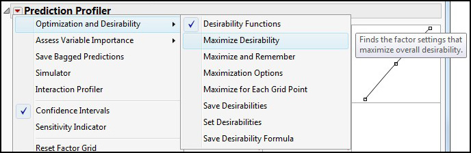
One of our objectives was to determine the settings for these three variables that would maximize the plant height. This is accomplished by activating the Desirability functions under the Little Red Triangle of the Prediction Profiler (Figure 16.27).

Figure 16.27: Activating the Desirability Functions

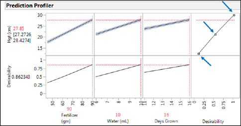
Since we set up the DOE with maximizing the height as the goal (Figure 16.15), JMP has remembered that, and the Desirability functions are already set up to maximize the height. This is accomplished by adjusting the three points (shown by blocks that can be clicked on and dragged to the desired setting) so that the maximum desirability of one is at the highest height and the lowest desirability approaching zero is at the lowest height (see arrows in Figure 16.28).

Figure 16.28: Optimizing Desirability

If your mouse hand is unsteady, or you are restricted to a touchscreen or touch pad such that it is difficult to catch and move the desirability dots to the desired location, you can also manually enter the numbers by calling up the Response Goal dialog box. Once again, the Little Red Triangle is your friend, and you can find the Set Desirabilities option second from the bottom of the Optimization and Desirability menu of the Prediction Profiler Little Red Triangle (Figure 16.27).

It is always a good idea to look at the optimization settings closely to see whether they make biological sense for the response being modeled. In this case, the optimum settings are the high setting for all three variables. Does it make biological sense that the highest amounts of fertilizer and water along with the longest growing time should yield the tallest plants? Almost any gardener or farmer would have no problem answering that! Of course, too high amounts of fertilizer and water are known to be detrimental for some plants, but in the data collected for the ranges tested here, that does not seem to be a problem.

Could this model be made any better? Remember that we have one interaction that is not contributing significantly to the model (Water * Days grown, p = 0.2735, Figure 16.24). What if we eliminated that variable from the model? And how does a main effects model compare to either of these with interactions? One of the great advantages of doing your statistics with software is that you can easily do these analyses in just a few minutes (if not seconds) and answer questions such as these. Using the metrics that allow us to determine the goodness of fit and to compare models as shown in Table 16.3, we can see that dropping the one interaction doesn’t really change much. The AICc is lower, and it is the simpler model that should predict just as well as the more complex model, and therefore would be the one to use for whatever conclusions are to be drawn for this experiment. In contrast, a main effects model is considerably poorer, having significant lack of fit and comparison metrics that clearly indicate that modeling with the main effects only is not a statistically satisfactory route to go.

Table 16.3: Comparing Models

Metric	ME + All three 2-way Interactions	ME + two 2-way interactions	Main Effects Only
LOF p-value	0.6331	0.5045	< 0.0001
RSqAdj	0.9907	0.9904	0.5524
AICc	42.3	36.0	88.3
BIC	27.9	27.4	86.2