Chapter 8: Tests on Frequencies: Odds Ratios and Relative Risk

If something has a 50% chance of happening, then 9 times out of 10 it will.

Yogi Berra (1925–2015)

Introduction

Experimental Design and Data Collection

Prospective Design

Retrospective Design

Relative Risk

Definition and Calculation

Interpretation of Relative Risk

Hormone Replacement Therapy: Yea or Nay?

Odds Ratios

Definition and Calculation

Interpretation of the Odds Ratio

Odds versus Probability

Renal Cell Cancer and Smoking

Introduction

In the previous chapter we saw how to detect the presence of a relationship between two variables with count or frequency data. But what if we find such a relationship and want to assess the strength of that association? Is there a metric we can calculate that will provide such a value? This is what we will consider in this chapter.

Consider the following abstract (underline added):

Background: HER2 positivity is reported to be <20% in gastric cancer. Clinicopathological characteristics will be helpful to understand the biological features of HER2-positive gastric cancer. Methods: A total of 813 gastric cancer patients who underwent HER2 testing between January 2005 and December 2010 were included in this study. Results: Ninety-five (11.7%) patients had HER2-positive gastric cancer. Elevated serum carcinoembryonic antigen (CEA) concentration [odds ratio (OR), 5.629; p < 0.001] and differentiated histology (OR, 3.717; p = 0.002) were significant predictive factors for HER2 positivity in localized disease. For recurrent or metastatic disease, elevated serum CEA concentration (OR, 2.545; p < 0.001), differentiated histology (OR, 3.299; p < 0.001), pulmonary metastasis (OR, 3.321; p = 0.001), and distant lymph node metastasis (OR, 2.286; p = 0.002) were significant predictive factors. Median disease-free survival (DFS) was shorter in HER2-positive patients than in others, especially in stage I or II disease (24.7 vs. 49.2 months; p < 0.001). Among HER2-negative patients with stage II diseases, patients who received adjuvant chemotherapy had longer DFS than others (42.2 vs. 30.7 months; p = 0.025). Conclusions: Clinicopathological factors may be useful in predicting the HER2 positivity of gastric cancer. Further studies are needed to understand the molecular basis of HER2-positive gastric cancer.1

In just this one example from the medical literature, we have the odds ratio used multiple times, and the ability to understand the results and conclusions is totally dependent upon the readers’ understanding of this metric. I use this abstract to point out to the premed students taking my course that even they need to know and understand biostatistics if they are to make intelligent decisions on the implications of medical research to their own medical practices. Odds ratios and relative risk are two of the more commonly used metrics that you will find in the biomedical literature for assessing the strength of the relationship between two variables. Usually, one variable is some measure of exposure to or treatment with something of interest to some disease state. But before we can dive into a description of these metrics, we need to take a side trip into the realm of experimental design.

Experimental Design and Data Collection

This is a classic case where how you collect the data determines how you can analyze the data, and how you collect the data is, in turn, an integral component of the experimental design. We must distinguish here between prospective and retrospective studies. They have both similarities and critical differences.

Prospective Design

To design a prospective study, the researcher collects two populations of subjects based on whether they are to receive an experimental treatment or have been exposed to a putative cause of the eventual outcome of interest to the experiment. So then, we have a treated or exposed experimental group and an untreated or unexposed control group to compare. The researcher then waits for a period of time and watches for the frequency of the outcome of interest in each group. Thus, he is looking forward in time from the initial creation of the two groups, that is, he is designing prospectively.

As an example of a prospective study, the case study that we will look at later in the chapter looks at whether women use hormone replacement therapy (HRT) and what impact such usage has on the outcome of death. Two groups of women were observed over time: one using and one not using HRT. The data collected is the count of those who die in the time period of interest. (More details when we look at these later.) The experimenters are seeking to determine if there is a relationship between the use of HRT and subsequent mortality.

Prospective studies are also called longitudinal or cohort studies. All three terms describe the same study design. The thing to remember here is that one can calculate either a relative risk or an odds ratio for this type of study design. Not so for the retrospective design.

Retrospective Design

In a retrospective study, the researcher again creates two populations of subjects, but this time, the subjects are divided based on whether they have the outcome of interest. The researcher then looks back, retrospectively, and determines the frequency of exposure to the risk factor (or treatment) in each of these groups. Usually, this can be accomplished by going to hospital records or some other database of personal information where the critical variables have been collected.

In other words, retrospective studies use pre-existing data to create two populations with and without the outcome of interest (usually a disease in this context) and then look back over the data previously collected to count within each of these two populations the frequency of exposure to a potential risk factor or causative agent. Clear as mud?

Retrospective studies are sometimes called case-control studies because the case subjects who have the outcome of interest are being compared to the control subjects who do not have the outcome of interest. Due to the nature of the data collection for this design, only odds ratios should be calculated for this type of experiment.

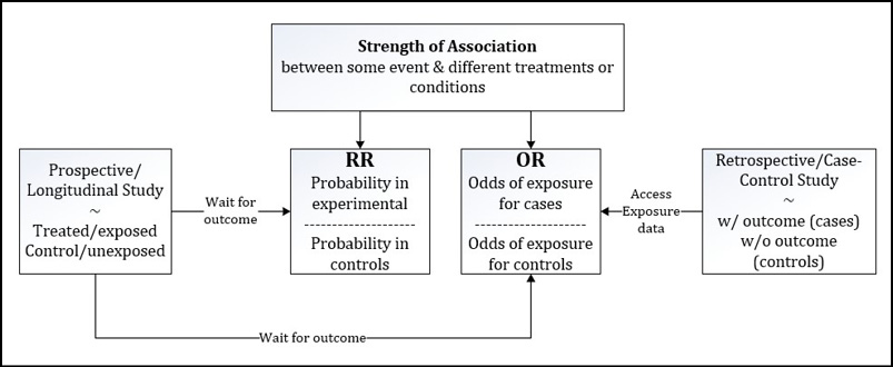
As we shall see later in this chapter, both types of experimental designs are analyzed as 2 x 2 contingency tables, so if the data is presented to the analyst in this format without any additional information, the type of design used to fill in the contingency table will need to be provided. That is to say, you cannot intuit the experimental design from just the data presentation. Both are presented in the same tabular format. Thus, the analyst must be told so that the correct metric can be used. (Alternatively, you can always calculate an odds ratio since that can be used for either design. But if relative risk is desired, the design should be prospective in nature.) Figure 8.1 gives a graphical representation and sets up our discussion of how to calculate each of these metrics in JMP.

Figure 8.1: Prospective Versus Retrospective Study Designs

Relative Risk

Definition and Calculation

The relative risk is simply the probability of the outcome of interest in the exposed group divided by the probability of the outcome of interest in the unexposed group. Figure 8.2 illustrates how to calculate this from the 2 x 2 contingency table.

Figure 8.2: Relative Risk Contingency Table and Formula

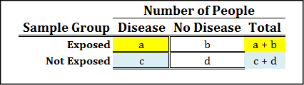
While you do not need to remember this formula because we are going to let JMP do the actual calculations for us, it is still helpful to have an idea of what it looks like, because it will help us interpret the value for the relative risk that is computed for any specific situation.

Interpretation of Relative Risk

Since relative risk is the ratio of the probability in the exposed group to the probability in the unexposed group, the null hypothesis would be no different between the two, and thus the ratio will have a value of one. This simply means that the treatment or exposure to a putative cause has no effect on the risk of disease or the outcome of interest. Given this definition, a relative risk greater than 1 means an increased risk of disease or the outcome of interest in the treated or exposed group. Likewise, a relative risk less than 1 means a decreased risk. The p-value associated with the relative risk will be the probability that the relative risk differs from a value of 1 (that is, the null hypothesis).

As a ratio, relative risk is a unitless number. However, it is frequently expressed as a percentage increase or decrease in the risk of the outcome using the following formula:

Relative Risk (Reduction or Increase)% = | 1 – RR | x 100

For example, a relative risk of 1.36 can be expressed as a 36% increase in the risk of a disease upon exposure to the risk factor of interest. This risk is always relative to the unexposed group, which is why it is called relative risk.

Take another example: what is the interpretation of a relative risk of 0.80? Answer: The risk of the outcome in the exposed group was reduced by 20% (or occurred 20% less) relative to the unexposed group.

Similarly, a relative risk of 3.30 means that the risk of the outcome in the exposed group was increased by 230% relative to the unexposed group. Or, one could also say that the outcome was 3.3 times more likely to occur in the exposed group than in the unexposed group.

Hormone Replacement Therapy: Yea or Nay?

Hormone replacement therapy (HRT) is frequently used in postmenopausal women to decrease the risk of cardiovascular disease and osteoporosis. Unfortunately, the use of HRT is also associated with an increased risk of breast and endometrial cancers. So, do the benefits outweigh the risks?

To answer this question, a subset of postmenopausal women was selected from the Nurses’ Health Study, a prospective study that was started in 1976 and updated every two years. Numerous variables are tracked in this database, providing a large data set for such investigations. Two of the variables tracked were the usage of HRT and mortality rates. The research question of interest can be phrased in this way: is there any evidence that the risk of death in women who were identified as currently using HRT relative to those who are not? (Note the italicized words in this phrasing. These will become important momentarily when we actually calculate the relative risk in JMP.) The data are in Table 8.1.2

Table 8.1: Contingency Table of HRT Data

	Number of People
	Deceased	Alive
Currently using HRT	574	8483
Never used HRT	2051	17520

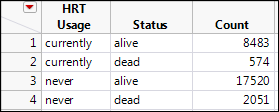
The first step is to translate this 2 x 2 contingency table into a JMP data table in which the count data is all in one column. Remember we have two categorical variables here, the HRT usage and the mortality outcome, so each should get their own column. Table 8.1 should be converted into the JMP table that looks like Figure 8.3.

Figure 8.3: HRT Usage Data Table

Since we are looking to determine if this data supports an association between these two variables, we need to do a chi-square test in the Fit Y by X platform. Click the Analyze menu option, then Fit Y by X, and fill out the subsequent form as found in Figure 8.4.

Figure 8.4: Fit Y by X Dialog Box Filled Out

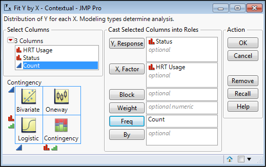
Because this is a prospective study, and the groups were initially separated based on HRT usage, that independent variable becomes our X, factor. The Status is the outcome of interest and that is our dependent Y, response. But most importantly, the Count column must be inserted into the Frequency input box (Freq). Failure to do this last step should be apparent when you look at the results of the analysis, which will be all ones in the resulting contingency table, and p-values of 1.0000 for the Chi-square p-values. If you see that, red flashing lights and sirens should go off in your head along with a loud monotone computer voice saying, “Error…Error…Error…” In short, don’t do that!

What should appear is the output seen in Figure 8.5.

Figure 8.5: Chi-Square Output of HRT Usage Data

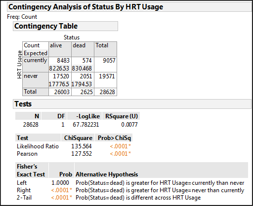
Let’s dissect out what this output is telling us. The contingency table allows us to compare our JMP data table to our initial data table to confirm that we have entered the right numbers for each of the variable combinations. The Pearson Chi-Square p-value of < .0001 tells us only that an association does, in fact, exist, but nothing more. Remember from the last chapter that this means the observed distribution of the counts in the different boxes of the contingency table is significantly different from those expected based on chance alone, that is, in the absence of an association between the two variables. The p-value tells us to reject the null hypothesis of no association, which means HRT usage does very significantly influence mortality in these women, but as yet we do not know if it is an increase or decrease in mortality (direction).

Fisher’s Exact Test allows us to determine the direction of the relationship. The right tailed test has the significant p-value, so we reject the null hypothesis represented by this one-sided test and accept the Alternative Hypothesis, which JMP helpfully provides for us in an abbreviated form. Reading this alternative hypothesis from left to right, we can translate it into “the probability of your status being ‘dead’ is greater if your HRT usage is ‘never’ relative to those currently using HRT.” So now we know, or can conclude that at least for this particular population of women, using hormone replacement therapy improved their chances of living longer.

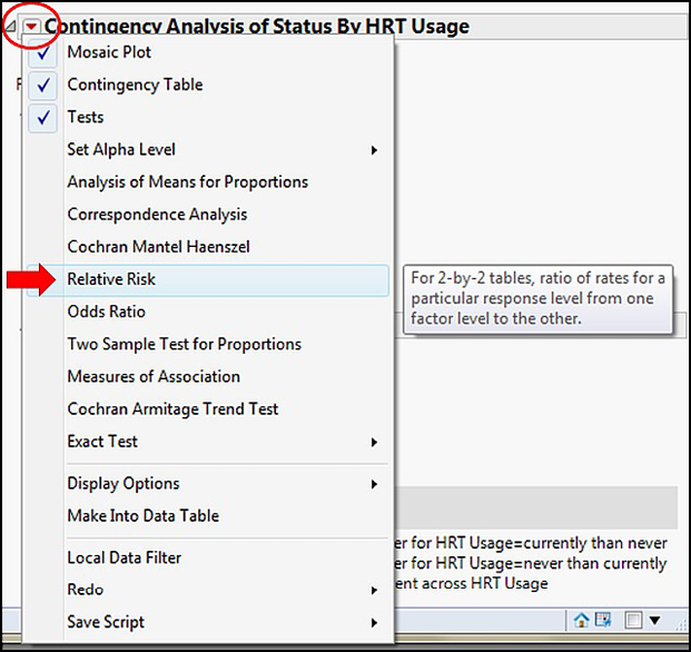
The final question is how much of an improvement can we expect? What is the relative risk quantitatively? Is the risk really that much better if HRT is used? In JMP, the Little Red Triangle Is Our Friend, and Relative Risk is found under our Friend as shown in Figure 8.6.

Figure 8.6: Locating Relative Risk in the Friendly Menu

There is a little bit of a hiccup here because selecting Relative Risk brings up this dialog box (Figure 8.7).

Figure 8.7: Special Relative Risk Questionnaire

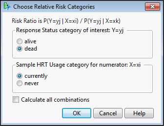
How the research question was phrased becomes important here. Or put another way, what is the specific relationship you are interested in? We want to know whether this data provides evidence that the risk of death (response = dead) differs in women identified as currently using HRT (Sample HRT Usage = currently) relative to those who are not, so the specific combination that we want is shown in Figure 8.7. You do have the option of selecting Calculate all combinations, and avoiding making this choice, but then you will still have to figure out which calculated relative risk best answers your question. It is really much better to reason it out with this dialog box and to resist the temptation to take what appears to be the easy way out and calculating them all. Either way, you have to think about what to actually use to draw your conclusion.

Selecting OK gives the output in Figure 8.8.

Figure 8.8: Relative Risk Output

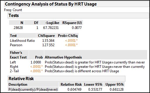
The relative risk calculation has been added to the bottom of the output already on your screen. We see we have a relative risk of 0.605 with a 95% confidence limit of 0.553 to 0.661. The good news is, the 95% confidence limit does not span a value of one, so this confirms the Pearson Chi-square p-value is showing a significant association between our variables. The value is less than one, so there is a decrease in risk, and reading the shorthand in the Description column and using our formula to convert to a percentage risk, we can conclude that there is a 40% reduction in risk of mortality (that is, of being “dead”) for women “currently” using HRT relative to those “never” using HRT in this population.

Odds Ratios

Definition and Calculation

As the name suggests, the odds ratio is a fraction just like the relative risk. However, in this case, it is the odds of exposure in those with the outcome divided by the odds of exposure in those without the outcome. Since the outcome is usually some disease state, we can define the odds ratio in other words as how many times more likely the odds are of finding an exposure to a risk factor in someone with the disease compared to finding an exposure in someone without the disease. The exposure can be to a risk factor, or it could be a treatment of some kind. Retrospective studies tend to be evaluating exposure to risk factors and prospective studies, to treatments. Thus, you can calculate an odds ratio once you have the data collected regardless of which study design was used to collect it.

Figure 8.9 shows the actual formula as related to the values in the 2 x 2 contingency table of the data.

Figure 8.9: Odds Ratio Contingency Table and Formula

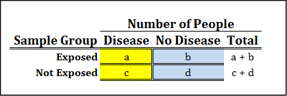
Interpretation of the Odds Ratio

An odds ratio of one means that there is no change in the frequency of exposure in the two populations, so this corresponds to the null hypothesis (similar to the relative risk). An odds ratio greater than one indicates there is an increased frequency of exposure among the case population, and contrariwise, an odds ratio less than one indicates there is a decreased frequency of exposure among the case population. Note how that is phrased. With odds ratios, we are talking about the odds of being exposed to a putative cause, not the odds of having the outcome if you had the exposure.

This difference is subtle, but important. Going back to the abstract with which we opened this chapter, the title of that paper is “Clinicopathological Features and Prognostic Significance of HER2 Expression in Gastric Cancer.” The outcome of interest is the presence of HER2 expression in the gastric cancer being examined because the expression of this gene has prognostic significance to the cancer patient. The first result cited in the Results section of the abstract indicates that “elevated serum carcinoembryonic antigen (CEA) concentration [odds ratio (OR), 5.629; p < 0.001]…[was a] significant predictive factor for HER2 positivity in localized disease.” The correct translation for this odds ratio: subjects that are HER2 positive for localized gastric cancer are 5.6 times more likely to have elevated CEA concentration, making elevated CEA concentrations a significant predictive factor in assessing HER2 positivity. Clear as mud?

Odds versus Probability

Before moving to an example, let’s briefly consider the difference between odds and probability. It is easiest to see the distinction with an example. Imagine a horse race where you expect the horse to win 5 races out of a total of 7 races. The odds the horse will win is the number of times you expect it to win divided by the number of times you expect it to lose. In our example, this would be 5/2 = 2 ½. We would probably say that the horse is two and a half times more likely to win than to lose. In contrast, the probability the horse will win is the fraction of times you expect the horse to win, which in this case is 5/7 = 0.71 or approximately 71% of the time. Both metrics are trying measure the same thing, but are essentially climbing the mountain from different sides.

Both the odds ratio and the relative risk are ratios, and both are trying to quantify the likelihood of an event (which corresponds to the strength of the association between the two variables in question). Many find relative risk ratios more intuitive than odds ratios, but that might merely be a matter of exposure and personal preference. As an interesting datum, when the disease is relatively rare, the odds ratio is close to the relative risk.

Renal Cell Cancer and Smoking

Cigarette smoking is associated with an increased incidence of many types of cancers. Investigators wanted to determine whether cigarette smoking was associated with an increased risk of renal cell cancer (RCC), so they constructed a retrospective case-control study. Control subjects without RCC were matched on sex, age (within 5 years), race, and neighborhood of residence to each case subject with RCC.3 After recruiting a total of 2314 subjects for the study, they visited them in their homes and interviewed them about their smoking habits (potential exposure variable) both past and present. The results are in Table 8.2.

Table 8.2: Renal Cell Cancer and Smoking Data

	Number of People
	RCC	No Cancer
Smoker	800	713
Never smoked	337	444

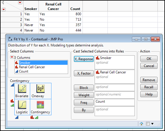
Here the independent variable is exposure to smoking, that is, are they a smoker or not (having never smoked at all). The dependent variable is whether they have RCC. However, notice how the data was collected. Being retrospective in nature, the initial groups were formed based on the experimental dependent variable, that is, their RCC status. When we set up our analysis in JMP, this variable becomes our X, factor instead of the Y, response that we would expect based on the cause-effect relationship we are trying to establish. Figure 8.10 shows the contingency table in Table 8.2 translated into a JMP data table with the Fit Y by X dialog box filled out for the correct analysis. Note again that the Count column must be assigned to the Freq box.

Figure 8.10: Renal Cell Cancer Data Table and Fit Y by X Dialog Box Filled Out

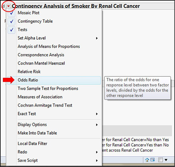
Once the initial analysis is complete, we must again resort to the Little Red Triangle. Astute observers may have noticed that the Odds Ratio was present in that menu back when we calculated the relative risk. Figure 8.11 shows us this menu.

Figure 8.11: Finding the Odds Ratio Option

The output in Figure 8.12 allows us to draw our conclusions.

Figure 8.12: Odds Ratio Output

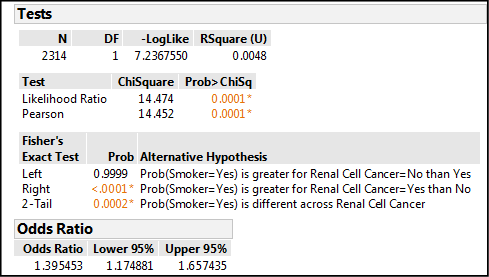
First, the p-value for the Pearson Chi-square test is 0.0001. This tells us there is an association between smoking and RCC, but not the direction or strength, only its presence. Next, the Fisher’s Exact Test gives us a significant p-value (< 0.0001) for the right sided test, so that is the alternative hypothesis supported by this data. Interpreting the JMP shorthand, the probability that a subject is a smoker (Smoker = yes) is greater for the group with RCC (Renal Cell Cancer = yes) than it is for those without RCC. This is logically and medically what we would expect. Lastly there is the odds ratio, which has a value of 1.395. We can see from the 95% confidence limits of the OR that one is not included in that range, which confirms our Pearson Chi-square conclusion: this odds ratio is significantly different from one. Therefore, there is something going on. The value is greater than one, so something has increased. In fact, this value tells us that individuals with RCC are 1.4 times more likely to be smokers than nonsmokers. We now have a quantitative metric for the strength of the association between smoking and renal cell cancer.