Search in book...
Toggle Font Controls
Create new playlist

Name your new playlist

Playlist description (optional)
Sign In

Email address

Password

Forgot Password?

or

Continue with Facebook

Continue with Google
Sign Up

Full Name

Email address

Confirm Email Address

Password

or

Continue with Facebook

Continue with Google

9.4 Factoring

We now turn to factoring. The basic method of dividing an integer $n$ $n$ by all primes $p \leq \sqrt{n}$ $p \leq \sqrt{n}$ is much too slow for most purposes. For many years, people have worked on developing more efficient algorithms. We present some of them here. In Chapter 21, we’ll also cover a method using elliptic curves, and in Chapter 25, we’ll show how a quantum computer, if built, could factor efficiently.

One method, which is also too slow, is usually called the Fermat factorization method. The idea is to express $n$ $n$ as a difference of two squares: $n = x^{2} - y^{2}$ $n = x^{2} - y^{2}$ . Then $n = (x + y) (x - y)$ $n = (x + y) (x - y)$ gives a factorization of $n$ $n$ . For example, suppose we want to factor $n = 295927$ $n = 295927$ . Compute $n + 1^{2}$ $n + 1^{2}$ , $n + 2^{2}$ $n + 2^{2}$ , $n + 3^{2}$ $n + 3^{2}$ , $\dots$ $\dots$ , until we find a square. In this case, $295927 + 3^{2} = 295936 = 544^{2}$ $295927 + 3^{2} = 295936 = 544^{2}$ . Therefore,

295927 = (544 + 3) (544 - 3) = 547 \cdot 541.

$295927 = (544 + 3) (544 - 3) = 547 \cdot 541.$

The Fermat method works well when $n$ $n$ is the product of two primes that are very close together. If $n = p q$ $n = p q$ , it takes $| p - q | / 2$ $| p - q | / 2$ steps to find the factorization. But if $p$ $p$ and $q$ $q$ are two randomly selected 300-digit primes, it is likely that $| p - q |$ $| p - q |$ will be very large, probably around 300 digits, too. So Fermat factorization is unlikely to work. Just to be safe, however, the primes for an RSA modulus are often chosen to be of slightly different sizes.

We now turn to more modern methods. If one of the prime factors of $n$ $n$ has a special property, it is sometimes easier to factor $n$ $n$ . For example, if $p$ $p$ divides $n$ $n$ and $p - 1$ $p - 1$ has only small prime factors, the following method is effective. It was invented by Pollard in 1974.

The $equation shows p1.$ $equation shows p1.$ Factoring Algorithm

Choose an integer $a > 1$ $a > 1$ . Often $a = 2$ $a = 2$ is used. Choose a bound $B$ $B$ . Compute $b \equiv a^{B!} (mod n)$ $b \equiv a^{B!} (mod n)$ as follows. Let $b_{1} \equiv a (mod n)$ $b_{1} \equiv a (mod n)$ and $b_{j} \equiv b_{j - 1}^{j} (mod n)$ $b_{j} \equiv b_{j - 1}^{j} (mod n)$ . Then $b_{B} \equiv b (mod n)$ $b_{B} \equiv b (mod n)$ . Let $d = gcd (b - 1, n)$ $d = gcd (b - 1, n)$ . If $1 < d < n$ $1 < d < n$ , we have found a nontrivial factor of $n$ $n$ .

Suppose $p$ $p$ is a prime factor of $n$ $n$ such that $p - 1$ $p - 1$ has only small prime factors. Then it is likely that $p - 1$ $p - 1$ will divide $B!$ $B!$ , say $B! = (p - 1) k$ $B! = (p - 1) k$ . By Fermat’s theorem, $b \equiv a^{B!} \equiv (a^{p - 1})^{k} \equiv 1 (mod p)$ $b \equiv a^{B!} \equiv (a^{p - 1})^{k} \equiv 1 (mod p)$ , so $p$ $p$ will occur in the greatest common divisor of $b - 1$ $b - 1$ and $n$ $n$ . If $q$ $q$ is another prime factor of $n$ $n$ , it is unlikely that $b \equiv 1 (mod q)$ $b \equiv 1 (mod q)$ , unless $q - 1$ $q - 1$ also has only small prime factors. If $d = n$ $d = n$ , not all is lost. In this case, we have an exponent $r$ $r$ (namely $B!$ $B!$ ) and an $a$ $a$ such that $a^{r} \equiv 1 (mod n)$ $a^{r} \equiv 1 (mod n)$ . There is a good chance that the $a^{r} \equiv 1$ $a^{r} \equiv 1$ method (explained later in this section) will factor $n$ $n$ . Alternatively, we could choose a smaller value of $B$ $B$ and repeat the calculation.

For an example, see Example 34 in the Computer Appendices.

How do we choose the bound $B$ $B$ ? If we choose a small $B$ $B$ , then the algorithm will run quickly but will have a very small chance of success. If we choose a very large $B$ $B$ , then the algorithm will be very slow. The actual value used will depend on the situation at hand.

In the applications, we will use integers that are products of two primes, say $n = p q$ $n = p q$ , but that are hard to factor. Therefore, we should ensure that $p - 1$ $p - 1$ has at least one large prime factor. This is easy to accomplish. Suppose we want $p$ $p$ to have around 300 digits. Choose a large prime $p_{0}$ $p_{0}$ , perhaps around $10^{140}$ $10^{140}$ . Look at integers of the form $k p_{0} + 1$ $k p_{0} + 1$ , with $k$ $k$ running through some integers around $10^{160}$ $10^{160}$ . Test $k p_{0} + 1$ $k p_{0} + 1$ for primality by the Miller-Rabin test, as before. On the average, this should produce a desired value of $p$ $p$ in less than 400 steps. Now choose a large prime $q_{0}$ $q_{0}$ and follow the same procedure to obtain $q$ $q$ . Then $n = p q$ $n = p q$ will be hard to factor by the $p - 1$ $p - 1$ method.

The elliptic curve factorization method (see Section 21.3) gives a generalization of the $p - 1$ $p - 1$ method. However, it uses some random numbers near $p - 1$ $p - 1$ and only requires at least one of them to have only small prime factors. This allows the method to detect many more primes $p$ $p$ , not just those where $p - 1$ $p - 1$ has only small prime factors.

9.4.1 $x superscript of 2 trible bond y superscript of 2.$ $x superscript of 2 trible bond y superscript of 2.$

Since it is the basis of the best current factorization methods, we repeat the following result from Section 9.4.

Basic Principle

Let $n$ $n$ be an integer and suppose there exist integers $x$ $x$ and $y$ $y$ with $x^{2} \equiv y^{2} (mod n)$ $x^{2} \equiv y^{2} (mod n)$ , but $x \equiv \pm y (mod n)$ $x \equiv \pm y (mod n)$ . Then $n$ $n$ is composite. Moreover, $gcd (x - y, n)$ $gcd (x - y, n)$ gives a nontrivial factor of $n$ $n$ .

For an example, see Example 33 in the Computer Appendices.

How do we find the numbers $x$ $x$ and $y$ $y$ ? Let’s suppose we want to factor $n = 3837523$ $n = 3837523$ . Observe the following:

\begin{array}{rcl} 9398^{2} & \equiv & 5^{5} \cdot 19 (mod 3837523) \\ 19095^{2} & \equiv & 2^{2} \cdot 5 \cdot 11 \cdot 13 \cdot 19 (mod 3837523) \\ 1964^{2} & \equiv & 3^{2} \cdot 13^{3} (mod 3837523) \\ 17078^{2} & \equiv & 2^{6} \cdot 3^{2} \cdot 11 (mod 3837523) . \end{array}

$\begin{array}{rcl} 9398^{2} & \equiv & 5^{5} \cdot 19 (mod 3837523) \\ 19095^{2} & \equiv & 2^{2} \cdot 5 \cdot 11 \cdot 13 \cdot 19 (mod 3837523) \\ 1964^{2} & \equiv & 3^{2} \cdot 13^{3} (mod 3837523) \\ 17078^{2} & \equiv & 2^{6} \cdot 3^{2} \cdot 11 (mod 3837523) . \end{array}$

If we multiply the relations, we obtain

\begin{array}{rcl} (9398 \cdot 19095 \cdot 1964 \cdot 17078)^{2} & \equiv & (2^{4} \cdot 3^{2} \cdot 5^{3} \cdot 11 \cdot 13^{2} \cdot 19)^{2} \\ 2230387^{2} & \equiv & 2586705^{2} . \end{array}

$\begin{array}{rcl} (9398 \cdot 19095 \cdot 1964 \cdot 17078)^{2} & \equiv & (2^{4} \cdot 3^{2} \cdot 5^{3} \cdot 11 \cdot 13^{2} \cdot 19)^{2} \\ 2230387^{2} & \equiv & 2586705^{2} . \end{array}$

Since $2230387 \equiv \pm 2586705 (mod 3837523)$ $2230387 \equiv \pm 2586705 (mod 3837523)$ , we now can factor 3837523 by calculating

gcd (2230387 - 2586705, 3837523) = 1093.

$gcd (2230387 - 2586705, 3837523) = 1093.$

The other factor is $3837523 / 1093 = 3511$ $3837523 / 1093 = 3511$ .

Here is a way of looking at the calculations we just did. First, we generate squares such that when they are reduced mod $n = 3837523$ $n = 3837523$ they can be written as products of small primes (in the present case, primes less than 20). This set of primes is called our factor base. We’ll discuss how to generate such squares shortly. Each of these squares gives a row in a matrix, where the entries are the exponents of the primes 2, 3, 5, 7, 11, 13, 17, 19. For example, the relation $17078^{2} \equiv 2^{6} \cdot 3^{2} \cdot 11 (mod 3837523)$ $17078^{2} \equiv 2^{6} \cdot 3^{2} \cdot 11 (mod 3837523)$ gives the row 6, 2, 0, 0, 1, 0, 0, 0.

In addition to the preceding relations, suppose that we have also found the following relations:

\begin{array}{rcl} 8077^{2} & \equiv & 2 \cdot 19 (mod 3837523) \\ 3397^{2} & \equiv & 2^{5} \cdot 5 \cdot 13^{2} (mod 3837523) \\ 14262^{2} & \equiv & 5^{2} \cdot 7^{2} \cdot 13 (mod 3837523) . \end{array}

$\begin{array}{rcl} 8077^{2} & \equiv & 2 \cdot 19 (mod 3837523) \\ 3397^{2} & \equiv & 2^{5} \cdot 5 \cdot 13^{2} (mod 3837523) \\ 14262^{2} & \equiv & 5^{2} \cdot 7^{2} \cdot 13 (mod 3837523) . \end{array}$

We obtain the matrix

\begin{matrix} 9398 \\ 19095 \\ 1964 \\ 17078 \\ 8077 \\ 3397 \\ 14262 \end{matrix} |\begin{array}{cccccccc} 0 & 0 & 5 & 0 & 0 & 0 & 0 & 1 \\ 2 & 0 & 1 & 0 & 1 & 1 & 0 & 1 \\ 0 & 2 & 0 & 0 & 0 & 3 & 0 & 0 \\ 6 & 2 & 0 & 0 & 1 & 0 & 0 & 0 \\ 1 & 0 & 0 & 0 & 0 & 0 & 0 & 1 \\ 5 & 0 & 1 & 0 & 0 & 2 & 0 & 0 \\ 0 & 0 & 2 & 2 & 0 & 1 & 0 & 0 \end{array}| .

$\begin{matrix} 9398 \\ 19095 \\ 1964 \\ 17078 \\ 8077 \\ 3397 \\ 14262 \end{matrix} |\begin{array}{cccccccc} 0 & 0 & 5 & 0 & 0 & 0 & 0 & 1 \\ 2 & 0 & 1 & 0 & 1 & 1 & 0 & 1 \\ 0 & 2 & 0 & 0 & 0 & 3 & 0 & 0 \\ 6 & 2 & 0 & 0 & 1 & 0 & 0 & 0 \\ 1 & 0 & 0 & 0 & 0 & 0 & 0 & 1 \\ 5 & 0 & 1 & 0 & 0 & 2 & 0 & 0 \\ 0 & 0 & 2 & 2 & 0 & 1 & 0 & 0 \end{array}| .$

Now look for linear dependencies mod 2 among the rows. Here are three of them:

$1st + 5th + 6th = (6,0,6,0,0,2,0,2) \equiv 0 (mod 2)$ $1st + 5th + 6th = (6,0,6,0,0,2,0,2) \equiv 0 (mod 2)$
$1st + 2nd + 3rd + 4th = (8,4,6,0,2,4,0,2) \equiv 0 (mod 2)$ $1st + 2nd + 3rd + 4th = (8,4,6,0,2,4,0,2) \equiv 0 (mod 2)$
$3rd + 7th = (0,2,2,2,0,4,0,0) \equiv 0 (mod 2)$ $3rd + 7th = (0,2,2,2,0,4,0,0) \equiv 0 (mod 2)$

When we have such a dependency, the product of the numbers yields a square. For example, these three yield

$(9398 \cdot 8077 \cdot 3397)^{2} \equiv 2^{6} \cdot 5^{6} \cdot 13^{2} \cdot 19^{2} \equiv (2^{3} \cdot 5^{3} \cdot 13 \cdot 19)^{2}$ $(9398 \cdot 8077 \cdot 3397)^{2} \equiv 2^{6} \cdot 5^{6} \cdot 13^{2} \cdot 19^{2} \equiv (2^{3} \cdot 5^{3} \cdot 13 \cdot 19)^{2}$
$(9398 \cdot 19095 \cdot 1964 \cdot 17078)^{2} \equiv (2^{3} \cdot 3^{2} \cdot 5^{3} \cdot 11 \cdot 13^{2} \cdot 19)^{2}$ $(9398 \cdot 19095 \cdot 1964 \cdot 17078)^{2} \equiv (2^{3} \cdot 3^{2} \cdot 5^{3} \cdot 11 \cdot 13^{2} \cdot 19)^{2}$
$(1964 \cdot 14262)^{2} \equiv (3 \cdot 5 \cdot 7 \cdot 13^{2})^{2}$ $(1964 \cdot 14262)^{2} \equiv (3 \cdot 5 \cdot 7 \cdot 13^{2})^{2}$

Therefore, we have $x^{2} \equiv y^{2} (mod n)$ $x^{2} \equiv y^{2} (mod n)$ for various values of $x$ $x$ and $y$ $y$ . If $x \equiv \pm y (mod n)$ $x \equiv \pm y (mod n)$ , then $gcd (x - y, n)$ $gcd (x - y, n)$ yields a nontrivial factor of $n$ $n$ . If $x \equiv \pm y (mod n)$ $x \equiv \pm y (mod n)$ , then usually $gcd (x - y, n) = 1$ $gcd (x - y, n) = 1$ or $n$ $n$ , so we don’t obtain a factorization. In our three examples, we have

$3590523^{2} \equiv 247000^{2}$ $3590523^{2} \equiv 247000^{2}$ , but $3590523 \equiv - 247000 (mod 3837523)$ $3590523 \equiv - 247000 (mod 3837523)$
$2230387^{2} \equiv 2586705^{2}$ $2230387^{2} \equiv 2586705^{2}$ and $gcd (2230387 - 2586705, 3837523) = 1093$ $gcd (2230387 - 2586705, 3837523) = 1093$
$1147907^{2} \equiv 17745^{2}$ $1147907^{2} \equiv 17745^{2}$ and $gcd (1147907 - 17745, 3837523) = 1093$ $gcd (1147907 - 17745, 3837523) = 1093$

We now return to the basic question: How do we find the numbers 9398, 19095, etc.? The idea is to produce squares that are slightly larger than a multiple of $n$ $n$ , so they are small mod $n$ $n$ . This means that there is a good chance they are products of small primes. An easy way is to look at numbers of the form $[\sqrt{i n} + j]$ $[\sqrt{i n} + j]$ for small $j$ $j$ and for various values of $i$ $i$ . Here $[x]$ $[x]$ denotes the greatest integer less than or equal to $x$ $x$ . The square of such a number is approximately $i n + 2 j \sqrt{i n} + j^{2}$ $i n + 2 j \sqrt{i n} + j^{2}$ , which is approximately $2 j \sqrt{i n} + j^{2}$ $2 j \sqrt{i n} + j^{2}$ mod $n$ $n$ . As long as $i$ $i$ is not too large, this number is fairly small, hence there is a good chance it is a product of small primes.

In the preceding calculation, we have $8077 = [\sqrt{17 n} + 1]$ $8077 = [\sqrt{17 n} + 1]$ and $9398 = [\sqrt{23 n} + 4]$ $9398 = [\sqrt{23 n} + 4]$ , for example.

The method just used is the basis of many of the best current factorization methods. The main step is to produce congruence relations

x^{2} \equiv product of small primes.

$x^{2} \equiv product of small primes.$

An improved version of the above method is called the quadratic sieve. A recent method, the number field sieve, uses more sophisticated techniques to produce such relations and is somewhat faster in many situations. See [Pomerance] for a description of these two methods and for a discussion of the history of factorization methods. See also Exercise 52.

Once we have several congruence relations, they are put into a matrix, as before. If we have more rows than columns in the matrix, we are guaranteed to have a linear dependence relation mod 2 among the rows. This leads to a congruence $x^{2} \equiv y^{2} (mod n)$ $x^{2} \equiv y^{2} (mod n)$ . Of course, as in the case of 1st + 5th + 6th $\equiv 0 (mod 2)$ $\equiv 0 (mod 2)$ considered previously, we might end up with $x \equiv \pm y$ $x \equiv \pm y$ , in which case we don’t obtain a factorization. But this situation is expected to occur at most half the time. So if we have enough relations – for example, if there are several more rows than columns – then we should have a relation that yields $x^{2} \equiv y^{2}$ $x^{2} \equiv y^{2}$ with $x \equiv \pm y$ $x \equiv \pm y$ . In this case $gcd (x - y, n)$ $gcd (x - y, n)$ is a nontrivial factor of $n$ $n$ .

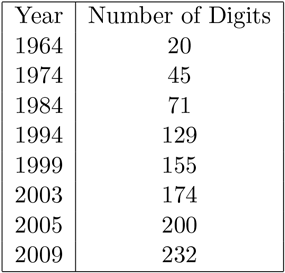
In the last half of the twentieth century, there was dramatic progress in factoring. This was partly due to the development of computers and partly due to improved algorithms. A major impetus was provided by the use of factoring in cryptology, especially the RSA algorithm. Table 9.2 gives the factorization records (in terms of the number of decimal digits) for various years.

A table summarizes the information of Factorization Records.

Table 9.2 Full Alternative Text

9.4.2 Using $equation ar trible bond 1.$ $equation ar trible bond 1.$

On the surface, the Miller-Rabin test looks like it might factor $n$ $n$ quite often; but what usually happens is that $b_{k - 1}$ $b_{k - 1}$ is reached without ever having $b_{u} \equiv \pm 1 (mod n)$ $b_{u} \equiv \pm 1 (mod n)$ . The problem is that usually $a^{n - 1} \equiv 1 (mod n)$ $a^{n - 1} \equiv 1 (mod n)$ . Suppose, on the other hand, that we have some exponent $r$ $r$ , maybe not $n - 1$ $n - 1$ , such that $a^{r} \equiv 1 (mod n)$ $a^{r} \equiv 1 (mod n)$ for some $a$ $a$ with $gcd (a, n) = 1$ $gcd (a, n) = 1$ . Then it is often possible to factor $n$ $n$ .

$equation a trible bond 1.$ $equation a trible bond 1.$ Factorization Method

Suppose we have an exponent $r > 0$ $r > 0$ and an integer $a$ $a$ such that $a^{r} \equiv 1 (mod n)$ $a^{r} \equiv 1 (mod n)$ . Write $r = 2^{k} m$ $r = 2^{k} m$ with $m$ $m$ odd. Let $b_{0} \equiv a^{m} (mod n)$ $b_{0} \equiv a^{m} (mod n)$ , and successively define $b_{u + 1} \equiv b_{u}^{2} (mod n)$ $b_{u + 1} \equiv b_{u}^{2} (mod n)$ for $0 \leq u \leq k - 1$ $0 \leq u \leq k - 1$ . If $b_{0} \equiv 1 (mod n)$ $b_{0} \equiv 1 (mod n)$ , then stop; the procedure has failed to factor $n$ $n$ . If, for some $u$ $u$ , we have $b_{u} \equiv - 1 (mod n)$ $b_{u} \equiv - 1 (mod n)$ , stop; the procedure has failed to factor $n$ $n$ . If, for some $u$ $u$ , we have $b_{u + 1} \equiv 1 (mod n)$ $b_{u + 1} \equiv 1 (mod n)$ but $b_{u} \equiv \pm 1 (mod n)$ $b_{u} \equiv \pm 1 (mod n)$ , then $gcd (b_{u} - 1, n)$ $gcd (b_{u} - 1, n)$ gives a nontrivial factor of $n$ $n$ .

Of course, if we take $a = 1$ $a = 1$ , then any $r$ $r$ works. But then $b_{0} = 1$ $b_{0} = 1$ , so the method fails. But if $a$ $a$ and $r$ $r$ are found by some reasonably sensible method, there is a good chance that this method will factor $n$ $n$ .

This looks very similar to the Miller-Rabin test. The difference is that the existence of $r$ $r$ guarantees that we have $b_{u + 1} \equiv 1 (mod n)$ $b_{u + 1} \equiv 1 (mod n)$ for some $u$ $u$ , which doesn’t happen as often in the Miller-Rabin situation. Trying a few values of $a$ $a$ has a very high probability of factoring $n$ $n$ .

Of course, we might ask how we can find an exponent $r$ $r$ . Generally, this seems to be very difficult, and this test cannot be used in practice. However, it is useful in showing that knowing the decryption exponent in the RSA algorithm allows us to factor the modulus. Moreover, if a quantum computer is built, it will perform factorizations by finding such an exponent $r$ $r$ via its unique quantum properties. See Chapter 25.

For an example for how this method is used in analyzing RSA, see Example 32 in the Computer Appendices.

..................Content has been hidden....................

You can't read the all page of ebook, please click here login for view all page.

Table of Contents for
9.4 Factoring

9.4 Factoring

The $equation shows p1.$ $equation shows p1.$ Factoring Algorithm

9.4.1 $x superscript of 2 trible bond y superscript of 2.$ $x superscript of 2 trible bond y superscript of 2.$

Basic Principle

Table 9.2 Factorization Records

9.4.2 Using $equation ar trible bond 1.$ $equation ar trible bond 1.$

$equation a trible bond 1.$ $equation a trible bond 1.$ Factorization Method

Table of Contents for 9.4 Factoring

Create new playlist

Sign In

Sign Up

Table of Contents for
9.4 Factoring