Chapter 6
Interpreting and using the solution of a linear programming model
6.1 Validating a model
Having built a linear programming model we should be very careful before we rely too heavily on the answers it produces. Once a model has been built and converted into the format necessary for the computer program we will wish to attempt to solve it. Assuming that there are no obvious clerical or keying errors (which are usually detected by package programs) there are three possible outcomes: (i) the model is infeasible; (ii) the model is unbounded; (iii) the model is solvable.
6.1.1 Infeasible models
A linear programming model is infeasible if the constraints are self-contradictory. For example, a model which contained the following two constraints would be infeasible:
6.1 ![]()
6.2 ![]()
In practice, the infeasibility would probably be more disguised (unless it arose through a simple keying error). The program will probably go some way towards trying to solve the model until it detects that it is infeasible. Most package programs will print out the infeasible solution obtained at the point when the program gives up.
In most situations an infeasible model indicates an error in the mathematical formulation of the problem. It is, of course, possible that we are trying to devise some plan that is technologically impossible, but more usually we are modelling a situation where we know there should be a feasible solution. The detection of why a model is infeasible can be very difficult. If we have got the infeasible solution where the program gave up we can see which constraints are unsatisfied or which variables are negative in this solution. This may enable us to find the cause of infeasibility fairly easily. It is quite possible, however, that it will not help. The cause of infeasibility may be fairly subtle. For example, it is impossible to satisfy each of the following constraints in the presence of the other two:
6.4 ![]()
It might, however, be wrong to single out any one of Inequalities (6.3)-(6.5) as being an infeasible constraint. What is wrong is the mutual incompatibility of all three constraints.
Assuming that we are modelling a situation which we know to be realizable, it should be possible to construct a feasible (but probably non-optimal) solution to the situation. For example, in a product mix model such as that presented in Section 1.2 we could take a previous week's mix of products (assuming no capacity has since been reduced). If our model were a correct representation of the situation, it should be possible to substitute this constructed (or known) solution into all the constraints without breaking them. As our model admits no feasible solution, this substitution must violate some of the constraints in the model. Any constraints violated in this way must have been modelled wrongly. They are too restrictive and should be reconsidered.
6.1.2 Unbounded models
A linear programming model is said to be unbounded if its objective function can be optimized without limit, that is, for a maximization problem the objective function can be made as large as one wishes or, for a minimization problem, as small as one wishes. For example, the following trivial linear programming problem is unbounded as x1 + x2 can be made as large as we like without violating the constraint:
6.6 ![]()
6.7 ![]()
While a correctly formulated infeasible model is just possible as we might be trying to attain the unattainable, a correctly formulated unbounded model is very unlikely.
As with infeasible models, most package programs print a solution to an unbounded model before the optimization is terminated on it being seen that the model is unbounded. This solution can be of help in detecting what is wrong with the model. On the other hand, detection of unboundedness may well be as difficult as the detection of infeasibility. An infeasible model has constraints which are over restrictive whereas an unbounded model either has vital constraints unrepresented or insufficiently restrictive. Usually, certain physical constraints have not been modelled. These constraints may well be so obvious as to be forgotten. A very common type of constraint to omit is a material balance constraint such as that described in Section 3.3. This sort of constraint is easily overlooked. If such a constraint has been inadvertently overlooked, the solution which the package program prints before giving up can be of use in detecting it. A common sense examination of this solution may reveal that things do not ‘add up’, for example, we may find we are producing something without using any raw material.
In Section 6.2 we define an associated linear programming model for every model known as the dual model. This model can have important economic interpretations. If a model is unbounded the corresponding dual model is infeasible. It is therefore conceivable that a practical unbounded model might arise as the dual to an infeasible model where we were testing whether a certain course of action was or was not possible. Should a model be infeasible we should not assume that its dual will necessarily be unbounded. It is possible that the dual will also be infeasible.
6.1.3 Solvable models
Should a linear programming model be neither infeasible nor unbounded we will refer to it as solvable. When we obtain the optimal solution to such a model we clearly want to know if the answer is sensible. If it is not sensible then there must be something wrong with our model. The first approach should be to examine the optimal solution critically simply using common sense. This may well reveal an obvious nonsense which should enable us to detect and correct a modelling error.
Should the solution still appear sensible we could compare the optimal objective value with what we might expect in practice. If, in a maximization problem, this value is lower than we expect, we might suspect that our model is over restrictive, that is, some constraints are too severe. On the other hand, if the optimal objective is higher than we expect, we might suspect that our model is insufficiently restrictive, that is, that some constraints are too weak or have been left out. For minimization problems these conclusions would obviously be reversed. To give an example, suppose we were considering a product mix application such as that considered in Section 1.2. On solving the model we would obtain a maximum profit contribution. Suppose this profit contribution was lower than what we already knew we could attain, for example, suppose it was lower than what we obtained in a previous week (assuming there had been no subsequent cut-back in productive capacity). In this circumstance we would obviously suspect our model to be over restrictive. To find where the over severe constraints lay we could substitute our known better solution into the constraints of our model. Some of these constraints will obviously be violated and must therefore have been modelled incorrectly. Possibly we may find that there is some productive capacity which we were unaware of but is being used by the workforce. Our model, even though not yet correct, will already be proving valuable in helping to discover things we were unaware of.
Thinking again about our product mix model, suppose we find the reverse situation that the optimal objective value was greater than anything we knew we could possibly achieve. In this situation our model would obviously be under-restrictive. The approach here would be to subject the optimal solution proposed by the model to a very critical examination. This solution could be presented in an entirely non-technical manner as a proposed operating policy and the appropriate management asked to spell out why it was impossible. It should then be possible to use this information to modify constraints or add new constraints.
For situations such as the above, where we are modelling an existing situation, we obviously have the great advantage of the ‘feasible’ solutions suggested by the existing mode of operation. These solutions can be used to test and modify our model. For situations where we are using linear programming (or any other sort of model) to design a new situation, for example, decide where to set up new plant, there may be no obvious ‘feasible’ solutions to use. Testing the model may therefore be more difficult. It is still a good approach to try to obtain good common sense solutions by rule of thumb methods. These solutions may well reveal errors in our model and show how they may be corrected.
The value of optimizing an objective should be apparent in this discussion on the validation of linear programming models. By optimizing some quantity we would expect to be using certain resources (processing capacity, raw materials, manpower, etc.) to their limit. The resultant optimal solution suggested by the model would then be fairly likely to violate certain physical restrictions which had been ignored or modelled incorrectly and thereby highlight them. It is often desirable to solve the model a number of times with different (possibly contrived) objectives in order to test out as many constraints as possible. The value of optimizing an objective (and so using mathematical programming) where there is no real life objective should be apparent in validating and modifying a model.
It should be obvious from the foregoing discussion that the building and validation of a model should be a two-way process gradually converging on a more and more accurate representation of the situation being modelled. Unfortunately, this process is often ignored or neglected. It can be an extremely valuable activity leading to a much clearer understanding of what is being modelled. In many situations this greater understanding may be more valuable than even the optimal solution to the (validated) model.
It is often possible to build a model with error detection in mind. For example, suppose we wished to define the following constraint:
If there were any danger of this constraint being too severe and making the model infeasible, we could allow it to be violated at a certain high cost by rewriting it as
and giving u a negative (‘cost’) coefficient in the objective function, assuming the problem to be a maximization. For a minimization problem u would be given a positive (‘profit’) coefficient. In this way the constraint could no longer cause the model to be infeasible but the violation of the original constraint (6.8) would be indicated by u appearing in the solution. For certain applications it might be argued that (6.9) was a more correct formulation of the constraint anyway by, for example, allowing us to ‘buy in’ more resources if really needed at a certain cost rather than restricting us absolutely. This topic was discussed in more detail in Section 3.3.
Another device can be used to avoid unboundedness occurring in a model. Each variable can be given a (possibly very large) finite simple upper bound in the formulation. No variable could then exceed its upper bound but any variable which rose to its bound would be open to suspicion. This might then lead one more quickly to the cause of unboundedness in the model.
Finally the desirability of using matrix generators should be re-emphasized here. By automatically generating a model the possibility of error is greatly reduced. The validation process itself is greatly simplified as the input to the matrix generator is usually presented in a much more physically meaningful form than for a linear programming package.
6.2 Economic interpretations
It will be useful to relate the discussion in this section to a specific type of model rather than present the material more abstractly. We will use the small product mix example of Section 1.2 for this purpose. The model was
This problem was that of finding how much to make of five products (PROD 1, PROD 2, …, PROD 5) subject to two processing capacity limitations (grinding and drilling) and a manpower limitation. Practical problems will, of course, usually be much bigger and more complex. The interpretation of the solution and the derivation of extra ‘economic’ information is, however, well illustrated by this example. Other types of application (e.g. blending) will, of course, result in different interpretations being placed on this information. It should, however, be possible to relate this information to any real life application after following the discussion applied to the small example above. The practical problems presented in Part II provide an excellent means of relating such information to real life situations.
If the model above is solved (by, for example, the simplex algorithm) the optimal solution turns out to be
![]()
giving an objective value of £10.920, that is, we should make 12 of PROD 1, 7.2 of PROD 2 and none of the other products. This results in a total profit contribution (over a week) of £10.920.
It can easily be verified that the grinding and manpower capacities are fully exhausted but that there is slack drilling capacity. This information is usually given along with the rest of the solution when a package program is used.
It can fairly easily be shown (although it is beyond the scope of this book) that in a model with m linear constraints (including possibly simple upper bounds) and a linear objective one would never expect more than m of the variables to be non-zero in the optimal solution. In the example above one could therefore be sure that one need never produce more than three products.
In a problem of the above kind there is a considerable amount of extra economic information, which might be of interest. For example, we can obtain answers to the following questions:
This extra information is usually presented with the ordinary solution when a package program is used. The variables have, associated with them, quantities known as reduced costs which can be interpreted (in this application) as the necessary price increases. Each constraint has associated with it a quantity known as the shadow price which can be interpreted as the marginal effect of increases (or decreases) in the capacities.
It should be emphasized that when the simplex algorithm (or one of its variants) is used to solve a model reduced costs and shadow prices arise naturally out of the optimal solution and most package programs print this information. There is, however, an alternative, and very illustrative, way of deriving this economic information which helps to clarify its true meaning. This is through another associated linear programming model known as the dual model which will now be described.
6.2.1 The dual model
We will again use the product mix problem above to illustrate this discussion.
Suppose that an accountant were trying to value each of the resources of this problem (grinding, drilling and manpower capacities) in some way so as to give a minimal overall valuation to the factory compatible with the optimal production plan. Let us suppose that the valuations for each hour of each of the capacities were y1, y2 and y3 (measured in £). The objective would be
The accountant wishes to obtain values for y1, y2 and y3 which totally explain the optimal production pattern. It should be possible to impute the profit contribution obtained from each product produced to its usage of the three resources. We must ensure that the profit contribution for each unit of each product is totally ‘covered’ by its imputed value. For example each unit of PROD 1 has a profit contribution of £550. This must be totally accounted for by the ‘value’ of the 12 hours grinding capacity, 10 hours drilling capacity and 20 hours manpower capacity used in making this unit. As the values of an hour of each of these capacities are y1, y2 and y3 (in £) we have
The reason why ‘≥’ is used rather than ‘=’ in the above constraint will not be totally obvious to start with. It should, however, become apparent later.
Similar arguments will relate the hourly values y1, y2 and y3 to the unit profit contributions of each of the other products. This gives constraints (4.12)–(4.15):
6.12 ![]()
6.13 ![]()
6.14 ![]()
The objective (6.10) together with the constraints (6.11)-(6.15) give us another linear programming model. As with most linear programming models we will implicitly assume that the variables y1, y2 and y3 can only be non-negative. This new linear programming model is referred to as the dual of the original product mix model. In contrast the original model is usually referred to as the primal model.
The derivation of this model may appear somewhat contrived at first but should become more plausible once we examine its solution.
Solving this dual model by a suitable algorithm we obtain the optimal solution
![]()
giving an objective value of 10 920; that is, we should value each hour of grinding capacity at £6.25, each hour of drilling capacity at nothing and each hour of manpower capacity at £23.75. The total valuation of the factory is then £10 920.
We can immediately see some connections between this result and the optimal production plan for the original product mix model:
Let us examine the optimal solution to the dual problem further and see what it might suggest to an accountant about the production policy which the factory should pursue.
Each unit of PROD 1 contributes £550 to profit. It uses up, however, 12 hours of grinding capacity (valued at £6.25 per hour), 10 hours of drilling capacity (valued at nothing) and 20 hours of manpower capacity (valued at £23.75 per hour). The total value imputed to each unit of PROD 1 is therefore
![]()
that is, the profit of £550 which each unit of PROD 1 contributes is exactly explained by the value imputed to it by virtue of its usage of resources. If we regarded the dual variables y1, y2 and y3 as ‘costs’, that is, we charged PROD 1 for its usage of scarce resources then we would come to the conclusion that PROD 1 produced zero profit. In accounting terms this does not matter as these ‘costs’ are purely internal accounting devices.
Similarly we find that each unit of PROD 2 has an imputed value (or extra ‘cost’) of
![]()
showing that the £600 contribution to profit is exactly accounted for.
For each unit of PROD 3 we get an imputed value (or extra ‘cost’) of
![]()
This ‘cost’ exceeds its profit contribution by £125. An accountant would conclude that PROD 3 would ‘cost’ more (in terms of usage of scarce resources) than it would contribute to profit. He or she would therefore suggest that PROD 3 not be manufactured. We came to the same conclusion using our original primal model.
It can easily be verified that PROD 4 and PROD 5 have ‘costs’ which exceed their unit profit contributions by £231.25 and £368.75 respectively and should therefore not be produced.
We are now in a position to see why the ‘≥’ rather than ‘=’ constraints in the dual model are acceptable. If the total activity in the left-hand side (the ‘cost’) of a constraint in the dual model strictly exceeds the right-hand side coefficient (the profit contribution) we do not incur this excess cost by simply not manufacturing the corresponding product. This gives us a third connection between the optimal solutions to the dual and primal models:
Returning to our accountant's analysis of the problem using the valuations derived from the dual model we conclude that
(Strictly speaking the deduction of (b) is not quite valid. It is certainly true that a non-binding constraint implies a zero valuation. The converse cannot immediately be concluded, although it presents no difficulty here. This complication is referred to later.)
The accountant could therefore eliminate x3, x4 and x5 from the primal problem, ignore the second (drilling) constraint and treat the remaining two constraints as equations. This gives
6.16 ![]()
6.17 ![]()
Solving this pair of simultaneous equations gives us
![]()
that is, the accountant deduces the same production plan using his or her valuations for the three resources as we do from our ordinary (primal) linear programming model. In practice the derivation of these valuations (values of the dual variables) by the method we have suggested (building and solving the dual model) might be just as difficult as, or more difficult than, building and solving the original (primal) model. Our purpose is, however, to explain a useful concept. In practice one would not normally build or solve the dual model (although in some circumstances this model is easier to solve computationally and might be used for this reason).
The product mix model for which we constructed a dual model was a maximization with all constraints ‘≤’. For completeness we should define the dual corresponding to a more general model. It is convenient to regard all problems as maximizations. In order to cope with a minimization we can negate the objective function and maximize it. It is also possible to convert all the constraints to ‘≤’. We do not choose to do this as it is helpful to keep the original model close to its original form. The dual variable corresponding to a ‘≤’ constraint was a conventional non-negative linear programming variable. A ‘≥’ constraint can be dealt with by only allowing the dual variable to be non-positive. For an ‘=’ constraint we will allow the dual variable to be unrestricted in sign. Such a variable is sometimes known as a free variable.
There is a symmetry concerning duality which should be mentioned although its main interest is purely mathematical. The dual of a dual model gives the original model.
6.2.2 Shadow prices
The valuations (values of the dual variables) which we have obtained by this roundabout means are in fact the shadow prices which we referred to in the earlier part of this section. They arise naturally, as subsidiary information, out of the optimal solution to the primal model if the simplex algorithm is used. It would, often, in fact be possible to deduce the shadow prices from simply the optimal solution values of the variables by using an argument similar to the accountancy argument which we used above. We will not, however, discuss the derivation of the shadow prices any longer as most package programs present these values in the output of the optimal solution.
It can fairly easily be seen (although we do not do so in this book) that the values of the dual variables (the shadow prices) represent the effects of small changes on the right-hand side coefficients, that is, they are marginal valuations. For example, if we were to increase grinding capacity by a small amount Δ then the resultant increase in total profit (after rearranging our optimal production plan) would be £(6.25 × Δ). Similarly the decrease in total profit by reducing grinding capacity would be £(6.25 × Δ). There will usually be limits within which Δ can lie. These limits (ranges) are discussed in the next section. (Strictly speaking it is possible that one or both of these limits be zero. This complication is discussed later). It will also only be valid to interpret the shadow prices as referring to the effect of small changes on one of the right-hand side coefficients at a time, that is, we could not make small changes in two right-hand side coefficients simultaneously and conclude that the effect on total profit will be the sum of the shadow prices.
Shadow prices can be of considerable value in making investment decisions. For example, each extra hour of grinding capacity is worth £6.25 per week to the factory. This interpretation remains valid as long as we are permitted to increase our grinding capacity by a sufficient amount. In the next section we will see that this capacity can be increased up to 384 hours per week (its upper range) with each extra unit resulting in an extra £6.25 per week. The effect of increasing capacity beyond this upper range will result in a smaller (though not immediately predictable) extra profit per unit of increase. As we can increase grinding capacity up to 384 hours per week, enabling us to make an extra £600 of profit, we could decide whether it is worth investing in (or hiring) more grinding machines. We might compare this with the £23.75 which would result from each extra hour of manpower capacity (within the permitted range) and decide where limited funds might be invested to best effect.
The shadow price on a non-binding constraint such as that representing the drilling capacity is zero. As we might expect there is no value in increasing this capacity as we do not use all we have already.
Shadow prices are an example of ‘opportunity costs’. This is a concept which accountants are increasingly (although still too rarely) using. For example an increase in grinding capacity results in an increased opportunity to make more profit. Similarly a decrease in grinding capacity loses us some opportunity to make a profit. The shadow price represents the cost of the lost opportunity. Unlike some of the other costs which accountants use (such as average costs), opportunity costs are quite a sophisticated concept. They result from a careful weighing up of the demands which each product makes on the scarce resources and contributes to profit in return. As a consequence they take into account the alternative uses to which the resources may be put and the comparative values of these alternative uses. One would obviously expect such costs to be of more value than less sophisticated costs. Accountants are becoming increasingly interested in linear programming as a result. A good description of the application of linear programming to accountancy is given by Salkin and Kornbluth (1973).
Our discussion of the interpretation of shadow prices has been confined to our product mix application. For other applications it should be possible to deduce the correct interpretation by relating small changes in the right-hand side coefficients to the physical situation represented by the model. To help with any such interpretation we suggest meanings which might be attached to the different types of constraint described in Section 3.3.
6.2.3 Productive capacity constraints
These are the sort of constraints we have discussed above where the capacity may represent limited processing or manpower. The interpretation of the shadow prices on such constraints has been fully dealt with above.
6.2.4 Raw material availabilities
Suppose we have modelled limited raw material availabilities by constraints. Those raw materials which the model suggests be used to their limit will be represented by constraints generally (but not always) having a non-zero shadow price. This shadow price will indicate the value of acquiring more of the raw material (within the permitted ranges). Similarly it will represent the cost of cutting back on raw material. This shadow price may be very useful in helping to decide whether to purchase more of the raw material or not (at a certain cost).
6.2.5 Marketing demands and limitations
The interpretation of the shadow prices here will be the effect on the value of the objective of altering demands or limitations of the market, for example, forcing the factory to produce more or less, or increasing or decreasing the maximum market size. Such a figure can often usefully be compared with the cost of extra sales effort. Frequently such constraints will take the form of simple upper bounds, as discussed in Section 3.3. If such simple upper bounds are treated as such in the model, they will not appear as constraints and therefore have no shadow price. The desired interpretation can, however, be obtained from the reduced cost of the bounded variable as described below.
6.2.6 Material balance (continuity) constraints
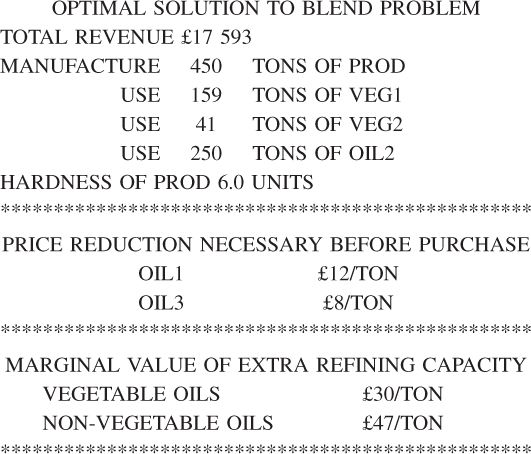
The shadow price on such constraints may well have no useful interpretation. For example, the small blending problem (Example 1.2) of Section 1.2 has a material balance constraint to make sure that the weight of the final product equals the total weight of the ingredients. The right-hand side value is zero. The shadow price predicts the effect of altering this zero value. It is hard to see a useful interpretation for this. In some circumstances the shadow price on a material balance constraint may be of interest. For example we may be equating our initial (or final) stocks to some expression involving the variables of the model. The shadow price will then indicate the effect on the optimal objective value of changing these stocks. A good example of this is the FOOD MANUFACTURE model of Part II.
6.2.7 Quality stipulations
Any model which involves blending as part of the total model usually involves quality stipulations, for example, the proportion of vitamins must not fall below a certain value or the octane rating of the petrol must not fall below some value. As an example, the blending problem in Section 1.2 has two quality constraints indicating a limitation on ‘hardness’. The shadow prices of these constraints can be used to predict the effect on total revenue of relaxing or tightening up on these hardness stipulations. In some models where the right-hand side coefficient is itself a quality parameter, the interpretation is straightforward. For our small example we had a right-hand side value of 0. The upper hardness constraint is
6.18 ![]()
Suppose this right-hand side coefficient were not 0 but were Δ. We could rewrite the constraint as
6.19 ![]()
In order to interpret the effect of a relaxing or tightening of the upper hardness limitation of 6, we would have to take into account the value of y in the optimal solution. A unit increase or decrease in the hardness 6 would result in an increase or decrease of y in the right-hand side and the interpretation of the shadow price would have to be adjusted accordingly. The derivation of ranges within which the hardness parameter could validly be altered with this interpretation would be difficult as the value of y would probably alter as well.
To decide whether a small change in a right-hand side coefficient results in an increase or decrease in the optimal objective value we should decide whether the change results in a relaxation or a tightening of the problem. If we relax a problem slightly, for example, increase the right-hand side coefficient on a ‘≤’ constraint or decrease the right-hand side coefficient on a ‘≥’ constraint, we would expect to at worse have no effect on the optimal objective value and perhaps improve it. Therefore the optimal objective value in a maximization problem would possibly get larger and in a minimization problem possibly get smaller, that is, we would expect to do no worse, possibly to do better in view of the lessening of the restrictions. For a tightening of the constraints, for example, reducing the right-hand side coefficients in a ‘≤’ constraint and increasing them in a ‘≥’ constraint, we would expect to do worse if anything, that is, possibly degrade the optimal objective value. In the case of ‘=’ constraints the improving or degrading effect of small changes in the right-hand side coefficient will probably be apparent from the meaning of the model.
Rather than formulate mathematical rules for interpreting whether the shadow price should be added or subtracted from the objective for each unit change in the corresponding right-hand coefficient it is probably better to follow the above scheme as different package programs vary in their sign conventions regarding shadow prices.
The suggested formulation of the TARIFF RATES (POWER GENERATION) problem in Part III causes the required rates for the sale of electricity to arise as shadow prices on demand constraints.
6.2.8 Reduced costs
In our small product mix example we saw that the unit profit contributions of PROD 1 and PROD 2 are exactly accounted for by the imputed ‘costs’ derived from the shadow prices on each constraint. For PROD 3, PROD 4 and PROD 5, however, the imputed costs exceed the unit profit contribution. The amount by which these unit profit contributions are exceeded in each case is of interest. These quantities are the reduced costs of these appropriate variables. Note that any variable which comes out at a non-zero level in the optimal solution has a zero reduced cost (this result is modified if the variable has a simple upper bound; the modification is dealt with later).
For our example the reduced costs which we derived earlier for PROD 3, and could also derive for PROD 4 and PROD 5 are
If we wanted to make PROD 3 we would have to increase its unit price by £125 before it was (just) worth making. This price increase would then allow the profit contribution of PROD 3 to balance the ‘costs’ imputed to it by way of its usage of scarce resources. Similarly, the reduced costs of PROD 4 and PROD 5 indicate price increases necessary for those products. The reduced costs are usually printed out with the solution values of the variables when a package program is used and there is no necessity to calculate them by way of the shadow prices as we have done. Our purpose in using this derivation has been to indicate the correct interpretation which should be placed on reduced costs. For other applications the interpretation of reduced costs will be different. In a blending problem for example (such as that in Section 1.2) the reduced costs might represent price decreases necessary before it became worth buying and incorporating an ingredient in a blend.
The above interpretation of reduced costs can be viewed the other way round. Suppose we insisted on making a small amount of PROD 3. As this will deny processing and manpower capacity to some of the other products (who could use it to better effect) we would expect to degrade our total profit. The amount by which this profit will be degraded for each unit of PROD 3 we make will be given by the reduced cost (£125) of PROD 3. In fact there will be a limit to the level at which PROD 3 can be made with this interpretation holding. This limit is another type of range which will be discussed in the next section. It is therefore possible to cost a non-optimal decision such as making PROD 3. This cost results from the lost opportunity to make other, more profitable, products. It is again an opportunity cost.
We should mention the slight variation in the interpretation of the reduced costs on variables with a finite simple upper bound as discussed in Section 3.3. If, in the optimal solution to a model, such a variable comes out at a value below its simple upper bound, there is no difficulty. The interpretation of the reduced cost will be exactly the same as that above. Suppose, however, that the variable were to come out at a value equal to its simple upper bound. This simple upper bound could well, in this case, be acting as a binding constraint. If the simple upper bound had been modelled as a conventional constraint, it would then have a non-zero shadow price which would be interpreted in the usual way. The variable would, being at a non-zero level, have a zero reduced cost. By modelling this constraint as a simple upper bound we will have lost the shadow price but it will appear as the reduced cost of the variable. The correct interpretation of this reduced cost will be the effect on the objective of forcing the variable down below its upper bound (degrading the objective) or increasing the upper bound (improving the objective).
We showed above how the shadow prices (values of the dual variables) could be used as ‘accounting costs’ in order to derive the optimal production plan in the product mix model. It is important to point out that such a procedure will not always work. This discussion also leads us on to an important feature of some linear programming models: alternative optimal solutions. Let us consider the following small linear programming model:
6.24 ![]()
If the dual model is formulated with dual variables y1, y2 and y3 corresponding to the three constraints, and then solved we obtain the following result:
![]()
An accountant could then use the values of y1, y2 and y3 as valuations for the constraints. This would lead the accountant to the following conclusions:
Suppose for the moment we did ignore constraints (6.21) and (6.23). We deduce that x1 and x2 must satisfy the equation
6.24 ![]()
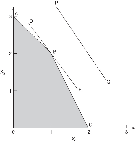
This equation obviously does not determine x1 and x2 uniquely. It is by no means obvious how the accountant should proceed from here. In fact it is impossible to deduce a unique solution to the above model from the solution to the dual model as the original (primal) model does not possess a unique solution. This is easily seen geometrically in Figure 6.1.
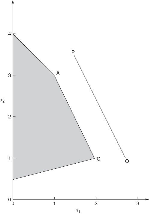
Different values of the objective function (6.20) correspond to different lines parallel to PQ. It so happens that PQ is parallel to the edge of AC of the feasible region created by constraint (6.22). We therefore see that any point on the line AC between (and including) A and C, gives an optimal solution to our model (objective = 7.5).
All that our accounting information has told us (if we ignore constraints (6.21) and (6.23)) is that 2x1 + x2 = 5, that is, that we must choose points lying on (or beyond) the line AC. We still have to pay some attention to the constraints (6.21) and (6.23). If we were to treat constraint (6.21) as binding we would arrive at the point A. Treating (6.23) as binding would give us point C. As mentioned in Section 2.2, the simplex algorithm only examines vertex solutions and would therefore choose either the solution at A (x1 = 1, x2 = 3) or the solution at C (x1 = 2, x2 = 1). Most package programs indicate when there are alternative solutions. They recognize this result by noticing one of the following properties of the optimal solutions:
In our example, if the optimal solution at A had been selected, we would note that constraint (6.21) was binding but had a zero shadow price. At C it would be constraint (6.23) that was binding with a zero shadow price.
It might seem rather unlikely that alternative solutions would arise in a practical linear programming model. In fact this is quite a common occurrence. For problems with more than two variables the situation will obviously be more complex. The characterization of all the optimal solutions (all vertex optimal solutions and various combinations of them) is often very difficult. It is, however, important to be able to recognize the phenomenon as if one optimal solution is unacceptable for some reason we have a certain flexibility to look for another solution without degrading our objective.
One of the purposes of this discussion has been to indicate that applying valuations (shadow prices) to the constraints of a linear programming model sometimes does not lead us to a unique solution (operating plan). The converse situation can also happen. We can have a unique solution (operating plan) determined by more than one set of valuations. For example, consider the following small problem:
6.25 ![]()
6.27 ![]()
6.30 ![]()
Let us attach valuations y1, y2, and y3 to each of the constraints (6.26)–(6.28). There are a number of valuations which will lead us to the optimal solution. For example,
Both these sets of valuations will lead us to the unique optimal solution to this problem:
![]()
giving an objective value of 7.
In a practical problem the question that would naturally arise is how should we derive a shadow price for our scarce resources given this ambiguity, for example, what would the value be of increasing the right-hand side value of 3 to 4? Would it be 1 or 0? This problem is again best illustrated by a diagram (Figure 6.2).
The constraints (6.26)–(6.28) give rise to the lines AB, BC and DBE respectively. Different objective values give rise to lines parallel to PQ, showing that B represents the optimal solution. The reason for the ambiguity in shadow price is that we have the ‘accidental’ result of three constraints going through the same point. Normally in two dimensions we would only expect two constraints to go through B. We can therefore regard either one of the constraints (6.26) or (6.28) as non-binding (having a zero valuation) in the presence of the other constraint. This leads to the ambiguity in our shadow prices.
In a situation such as this it would not be correct to increase the right-hand side value of 3 in constraint (6.26) at all using the shadow price of 1. The upper range of this right-hand side value (with this shadow price) will be 3. The coefficient is already at its upper range and any further increase will not alter the objective at the rate suggested by the valuation.
In these situations the shadow price is usually defined as being the rate of change of value of the objective function with respect to the right-hand side value. Then it can be shown that the upper shadow price (for increases in right-hand side value) is the minimum of all the possible valuations and the lower shadow price (for decreases in right-hand side value) is the maximum of all the possible valuations. Defining y1, y2, and y3 as shadow prices we have
When a computer package is used, the ‘shadow prices’ printed out are usually only the values of the dual variables corresponding to one dual solution. They are therefore misleading if interpreted as shadow prices according to the above definition. In fact to evaluate all the alternative dual solutions, and therefore obtain the true shadow price, would generally be computationally prohibitive. It is, however, possible to evaluate ranges within which the valuations associated with any particular dual solution chosen are valid. For example, the upper shadow price on constraint (6.26) is not 1. If we take the dual solution (i) above, then the associated upper range on the right-hand side coefficient of 3 is also 3, showing there is no range within which this coefficient can be increased to reflect a rate-of-change increase of 1 in the objective. This example is considered again in Section 6.3, when ranges are discussed. A good discussion of the problem is given by Aucamp and Steinberg (1982).
It should be pointed out that the two complications we have just discussed are dual situations. On the one hand we had a unique dual solution leading to more than one primal solution. The first phenomenon is referred to as alternative solutions (in the primal model) while the second phenomenon is referred to as degeneracy (in the primal model).
6.3 Sensitivity analysis and the stability of a model
6.3.1 Right-hand side ranges
In the last section we described how shadow prices can be useful in predicting the effect of small changes in the right-hand side coefficients on the optimal value of the objective function. It was pointed out, however, that this interpretation is only valid in a certain range. In this case the range is known as a right-hand side range. We will again use the product mix problem of Section 1.2 to illustrate our discussion. This gave the model
6.29 ![]()
6.31 ![]()
We saw that the optimal solution told us to make 12 of PROD 1 and 7.2 of PROD 2 and nothing of PROD 3, PROD 4 and PROD 5. This resulted in a profit of £10.920 and exhausted the grinding capacity (constraint (6.30)) and manpower capacity (constraint (6.32)).
The shadow prices on constraints (6.30)–(6.32) turned out to be 6.25, 0 and 23.75. Increasing the grinding capacity by Δ hours per week would therefore result in a weekly increase in a total profit of £(6.25 × Δ). Similarly, cutting back on grinding capacity by Δ hours per week would result in a weekly decrease in the total profit of £(6.25 × Δ). We are interested in the limits within which the change Δ can take place for this interpretation to apply. For this example these ranges are as follows:
![]()
that is, we can increase grinding capacity by up to 96 hours a week or decrease it by up to 57.6 hours per week with the predicted effect on profit. Changes outside these ranges are unpredictable in their effect and require further analysis. The information that we have got here is, however, of some, if limited, usefulness. It tells us, for instance, that adding one grinding machine would improve profit by £(96 × 6.25) = £600 per week. We could not, however, predict the effect on total profit of taking away a grinding machine as this would take us below the lower range of the grinding capacity. It would nevertheless be correct to say that £600 is, if anything, an underestimate for the resultant decrease in profit.
It is important to restate that this interpretation of the effect on the objective of decreasing or increasing a right-hand side coefficient is only valid if one coefficient is changed at a time within the permitted ranges. The effect of changing more than one coefficient at a time, as well as changes outside the permitted ranges, are efficiently examined by parametric programming, which is discussed in the next section.
It is beyond the scope of this book to describe how the right-hand side ranges are calculated. Most computer packages provide these ranges with their solution output.
For completeness we will give the upper and lower ranges on the other two capacities: drilling and manpower.
The ranges on the drilling capacity of 192 hours per week are fairly trivial to obtain. Remember that we are not using all our drilling capacity. In fact we have a slack capacity of 14.4 hours. This immediately enables us to calculate the lower range by subtracting this figure from the existing capacity. As we are not using all our drilling capacity, increasing it without limit can have no effect on the solution. The ranges are therefore
![]()
Within these ranges there will be no change at all in the objective (or optimal solution) as the shadow price on the (non-binding) drilling constraint is zero.
The ranges on the manpower capacity of 384 hours per week are again non-trivial to calculate. They turn out to be as follows:
![]()
For changes within these ranges the objective changes by £23.75 for each unit of change. For example an extra worker (48 hours per week) improves profit by (23.75 × 48) = £1140 per week. This might prove quite valuable information when compared with the fact that an extra grinding machine is worth only £600 per week.
The meaning of right-hand side ranges is well illustrated geometrically using a two-variable example:
6.33 ![]()
6.35 ![]()
6.39 ![]()
Geometrically we have the situation in Figure 6.3. The optimal solution is represented by the point A, giving an objective value of 9. The shadow price on constraint (6.34) turns out to be 1.
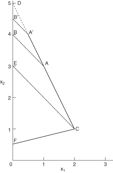
If constraint (6.34) is relaxed by increasing the right-hand side coefficient from 4 to 4.5 we move the boundary AB of the feasible region to A′B′. The resultant increase in the objective is 1 × 0.5 = 0.5. We can continue to increase the right-hand side coefficient to 5 when this boundary of the feasible region shrinks to the point D. There is clearly no virtue in further increasing the right-hand side coefficient as the point D will continue to represent the optimal solution. The upper range on the right-hand side coefficient in constraint (6.34) therefore is obviously 5.
If constraint (6.34) is tightened by decreasing the right-hand side coefficient, the boundary AB of the feasible region progressively moves down until it becomes CE. This happens when the right-hand side coefficient is 3. Any decreases in this coefficient between 4 and 3 result in a degradation of the objective by 1 (the shadow price) for each unit of decrease. The value 3 is the lower range. For decreases in coefficient values below 3 the optimal objective value will decrease at a greater rate. This rate will not immediately be predictable from our knowledge of the solution at A. For decreases down to 3 the optimal objective value is represented by points on the line AC. Decreases below 3 give points on the line CF.
So far we have only suggested using right-hand side ranges together with shadow prices to investigate the effect which changes on the right-hand side coefficients have on the optimal objective value. Such investigations sometimes give rise to the expression post-optimal analysis. Another purpose to which such information can be put is in investigating the sensitivity of the model to the right-hand side data. This forms part of a subject known as sensitivity analysis.
We will consider this new use to which right-hand side ranging information can be put in relation to the product mix model. Suppose we were rather doubtful about the accuracy of the grinding capacity of 288 hours per week (constraint (6.30)). In practice it is quite likely that such a figure would be open to doubt as machines could well be down for maintenance or repair for durations which were not wholly predictable. How confident should we be in suggesting that the factory dispenses with making PROD 3, PROD 4 and PROD 5 and only concentrates on PROD 1 and PROD 2? From our range information we can immediately say that this should remain the optimal policy as long as the true capacity figure does not lie outside the limits 230.4–384. Although the policy (in terms of what is, and is not, made) does not change within these limits, the levels at which PROD 1 and PROD 2 are made (and the resultant profit) obviously will change. This information is therefore of limited, but nevertheless sometimes significant, usefulness. Obviously if there is doubt about one capacity figure there will probably also be doubt about others and ranging information can only strictly be applied when one change only is made. Nevertheless such information does give some indication of the sensitivity of the solution to accuracy in the right-hand side data. If, for example, the ranges on the right-hand side coefficient in constraint (6.30) had been very close, say 287–288.5, we would have to be very careful in applying our suggested solution as it clearly would depend very critically on the accuracy of the grinding capacity figure.
It should be pointed out that the sensitivity analysis interpretation of the easily obtained ranges of 177.6 and ∞ on the non-binding drilling constraint is rather stronger. As long as this capacity lies within these figures not only will our optimal solution be no different, but the levels of the variables in that optimal solution will be unchanged as well.
Changing the right-hand side coefficient on a binding constraint within the permitted ranges does of course alter the values of the variables in the optimal solution (as well as the objective value). The rates at which the values of the variables change are quite easily obtained using most package programs. Such values are known as marginal rates of substitution and discussed below. Before doing this, however, we will consider other types of ranging information to be obtained from a linear programming model.
6.3.2 Objective ranges
It is often useful to know the effects of changes in the objective coefficients on the optimal solution. Suppose we change an objective coefficient (e.g. a unit profit contribution or cost). How will this affect the value of the objective function? In an analogous manner to right-hand side ranges we can define objective ranges. If a single objective coefficient is changed within these ranges then the optimal solution values of the variables will not change (although the optimal value of the objective may change). This is a rather stronger result than in the right-hand side ranging case where the solution values could change. The result is not altogether intuitive. If a particular item became more profitable or costly we might expect to bias our solution towards or away from that item. In fact our solution will not change at all as long as we remain within the permitted ranges. The situation is well described geometrically by means of the two-variable model we used before:
6.37 ![]()
6.38 ![]()
6.39 ![]()
6.40 ![]()
![]()
This gives rise to Figure 6.4. The optimal solution (x1 = 1, x2 = 3, objective = 9) is represented by the point A. The line PQ represents the points giving an objective value of 9.
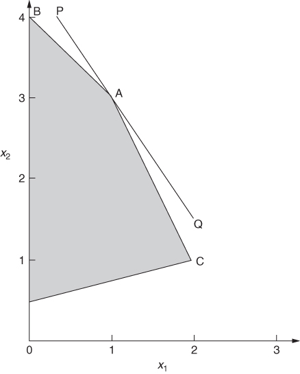
Suppose that the objective coefficient 3 of variable x1 were to increase. The steepness of the line PQ would increase (in a negative sense) but A would still represent the optimal solution as long as PQ did not rotate (around A) in a clockwise direction beyond the direction AC. When the objective coefficient of x1 became 4 the objective line would coincide with the line AC. This provides us with an upper range of 4 for this coefficient. Similarly a lower range is provided by decreasing this coefficient until the objective line coincides with AB. This gives a lower range of 2. Note that as long as the objective coefficient of x1 remains within the range 2–4, the optimal solution values of the variables will be unchanged and represented by point A. This is the slightly unintuitive result mentioned before. The optimal objective value does of course change if we alter this coefficient within its ranges. As x1 has a value of 1 in the optimal solution, each unit of increase or decrease in its objective coefficient will obviously provide an increase or decrease of 1 in the objective value.
Ranges on the objective coefficient of 2 for x2 can be discovered in a similar manner.
We will now return to our product mix example and present the objective ranges for that problem. To describe how these ranges are calculated in a problem which cannot be represented geometrically is beyond the scope of this book. Most package programs do, however, provide this information. Our main concern is with the correct interpretation rather than the derivation.
For PROD 1 the ranges on the objective coefficient are
![]()
This means that if we vary the objective coefficient of PROD 1 within these limits the values of the variables in our optimal solution will not change. We should still continue to produce 12 of PROD 1, 7.2 of PROD 2 and nothing else. As remarked before, such a result is often difficult for people with little understanding to accept. We might expect there to be a gradual and continuous shift towards making more of PROD 1, the more expensive we make it. In fact the production plan should not alter at all until PROD 1 produces a unit profit contribution of more than £600. When this happens there will be a new optimal production plan (almost certainly involving more of PROD 1) the investigation of which would require further analysis. The same restrictions apply to the interpretation of objective ranges as applied in the case of right-hand side ranges. Our interpretation is only valid within the permitted ranges and if only one change is made in an objective coefficient. This clearly limits the value of this information somewhat. Parametric programming provides an efficient means of investigating the effects of more than one change, possibly outside the ranges.
Although the optimal solution values of the variable do not change within the ranges, the objective value obviously will. For each £1 that we add to the price of PROD 1 we obviously improve the objective by £12 as the optimal solution involves producing 12 of PROD 1.
Similarly objective ranges can be obtained for PROD 2. These turn out to be
![]()
For PROD 3, PROD 4 and PROD 5, which should not be made in the optimal production plan, the derivation of objective ranges is simple. We have already seen that PROD 3 must be increased in price by £125 (its reduced cost) before it is worth making. This gives us its upper range. As it is already too cheap to be worth making a reduction in price cannot affect the solution. The objective ranges for PROD 3 are therefore
![]()
For PROD 4 we have
![]()
For PROD 5 we have
![]()
Objective ranges can be put to a similar use to that which right-hand side ranges are put in sensitivity analysis. If there were doubt surrounding the true profit contribution of £550 from PROD 1, we could be sure of our production plan as long as we knew that this figure was between £500 and £600. The width or narrowness of the objective ranges enables one to obtain a good feel for the sensitivity of the solution to changes (or errors in the objective data). In fact this interpretation is rather stronger than is the case with right-hand side ranges. Not only will the optimal production policy not change if a coefficient is altered within its permitted ranges; the values of the variable quantities in that plan will not alter either.
6.3.3 Ranges on interior coefficients
It is also possible to obtain ranges for other coefficients in a linear programming model. Sometimes these may provide valuable information in much the same way that right-hand side and objective ranges do. Generally, however, such information is far less useful. When a model is built often the only data which are changed are the objective and right-hand side coefficients (taken together these are sometimes referred to as the rim of the model). In consequence many package programs do not provide the facility for obtaining ranges on coefficients other than in the rim. When such information is obtainable its interpretation and use is very similar to that in the case of right-hand side and objective ranges.
We must now consider the complication which we described in Section 6.2 when there was ambiguity concerning the valuations (shadow prices) of the constraints. This ambiguity also extends to the ranging information. Alternative sets of valuations corresponding to a unique optimal solution lead to alternative sets of ranges. We will repeat the small example we used before:
6.41 ![]()
![]()
There are a number of possible valuations for the constraints which give rise to the optimal solution. We presented the following two where y1, y2 and y3 are the dual values on constraints (6.42)–(6.44), respectively:
(i) arises when we regard constraints (6.42) and (6.43) only as binding; (ii) arises when we regard constraints (6.43) and (6.44) only as binding.
Table 6.1 gives the right-hand side ranges within which the set (i) can be used as shadow prices.
| Constraint | Lower Range | Upper Range |
| 6.42 | 2 | 3 |
| 6.43 | 3 | 4 |
| 6.44 | 10 | ∞ |
Each range extends on one side of the right-hand side coefficient only. For example, constraint (6.42) has an upper range of 3, indicating that it would be incorrect to use a shadow price of 1 on this constraint to predict the effect of increasing the right-hand side coefficient. It would, however, be correct to use this as a shadow price to predict the effect of decreasing this coefficient. Similar arguments apply to the other two constraints. For constraint (6.44) we can increase the right-hand side coefficient of 10 indefinitely without affecting the optimal solution or objective value (shadow price of 0). We cannot, however, decrease this coefficient at all without altering the objective. This last result is obvious from studying Figure 6.2.
The clue to changes in the right-hand side coefficients in the other directions is given by the set of valuations (ii) together with their corresponding ranges. These ranges are given in Table 6.2. For example, increasing the right-hand side coefficient of 3 has no effect (shadow price of 0) on the objective whereas decreasing this coefficient does have an effect (shadow price of 1). Similarly the second set of ranges on the other constraints are in opposite directions indicating the ranges of interpretation of the second set as shadow prices.
| Constraint | Lower Range | Upper Range |
| 6.42 | 3 | ∞ |
| 6.43 | 4 | 5 |
| 6.44 | 8 | 10 |
We have demonstrated how two-valued shadow prices can exist for constraints with different marginal values for decreasing or increasing a right-hand side coefficient. In solving a practical model using a package program the user will only be presented with one set of ‘shadow prices’ corresponding to his or her optimal solution. Which set of dual values this is will be very arbitrary and depend upon the manner in which the model was solved. Solving the same model with exactly the same data could well result in a different set of dual values. The clue to the limited (one-sided) interpretation which can be placed on these shadow prices lies in the right-hand side ranges. If some of these ranges lie on one side of their corresponding right-hand side coefficient only, then this limits the shadow price to being interpreted for changes in one direction only. To investigate the effects of changes in the opposite direction alternate sets of dual values and their corresponding ranges should be sought. Alternatively parametric programming could be used as discussed in the next section.
It may well seem to the reader that a disproportionate amount of attention has been paid, in both this and the last section, to the apparently rather trivial complication concerning alternative valuations (shadow prices) for the constraints of a linear programming model. As has already been pointed out, however, this complication is a very common occurrence in practical linear programming models. It is well known in the computational side of linear programming as the phenomenon of degeneracy. We have here been concerned with the economic interpretations concerning degenerate solutions. In view of the difficulty which many people have in understanding this, we have given it considerable attention.
A further, rather different, final point should be made concerning the uniqueness of the ranging information from a model. The inclusion or exclusion of redundant constraints from a model will obviously not affect the optimal solution. This could well, however, affect the values of the ranges. Figure 6.3 and its associated model illustrate this point. Constraint (6.36) gives rise to the edge CF of the feasible region. The ignoring of constraint (6.36) would obviously not affect the optimal solution represented by the point A. In this sense constraint (6.36) is redundant and might never have been modelled in the first place in a practical situation if its redundancy had been obvious. The presence or absence of constraint (6.36) will, however, obviously affect the value of the lower right-hand side range on constraint (6.34). With constraint (6.36) present this lower range is 3. If constraint (6.36) were removed it would be 2.5.
6.3.4 Marginal rates of substitution
We have seen that there is a certain flexibility in altering a right-hand side coefficient of a model. As long as we remain with the permitted range the effect on the objective value is governed (for each unit of change) by the shadow price of the constraint. This change in the objective value occurs because the values of the variables in the optimal solution change. The relative rates at which they change are given by the marginal rates of substitution. It is beyond the scope of this book to describe how these figures can be calculated but they are obtainable from the solution output of most package programs. A small geometric example will illustrate the meaning which should be attached to these figures. Our example is the same as that used before:
6.46 ![]()
6.47 ![]()
![]()
The feasible region is represented by Figure 6.5. The optimal solution is represented by point A (x1 = 1, x2 = 3 objective = 9).
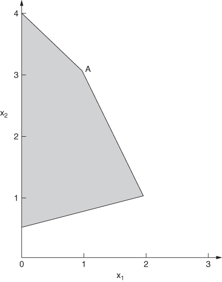
We have already seen that the right-hand side coefficient of 4 on constraint (6.45) can be changed within the range 3–5, causing the objective to change by 1 (the shadow price on constraint (6.45)) for each unit of change. The values of the variables (x1 and x2) will also obviously change. Their rates of change, per unit increase in this right-hand side coefficient, are
| x1 | –1 |
| x2 | + 2 |
that is, x1 will get smaller by one and x2 will get larger by two for each unit of increase. Decreasing the right-hand side coefficient will obviously produce the opposite effect.
Such figures can be very valuable in many applications. For example, they might indicate how a production plan should alter as a certain resource becomes scarcer or more plentiful. In a blending application they could indicate the rate at which one ingredient should be substituted for another as it became more plentiful.
The same limitations apply to the interpretation of marginal rates of substitution as apply to shadow prices. We can only consider one change at a time within the permitted ranges. If a range is one-sided we can only apply the marginal rates of substitution for changes in one direction. A different set of marginal rates of substitution will exist (although it will require more computation to derive) for changes in the opposite direction.
The subjects of sensitivity and post-optimal analysis are fully covered in the papers of Greenberg (1993a, 1993b, 1993c, 1994).
6.3.5 Building stable models
We have shown that quite a lot of useful information can be obtained to suggest how sensitive the optimal solution to a linear programming model is to changes (or inaccuracies) in the data. In many practical situations stable solutions are more valuable than optimal solutions. Having obtained an optimal solution to a model we might be very reluctant to change our operating plan if only small changes occurred in certain parameters, for example, capacities or costs. To some extent we can incorporate this reluctance in our model.
Suppose we were to run out of a particular resource (e.g. processing capacity, raw material, and manpower). It might well be that in practice we would buy in more in this resource at a cost until this increased cost became prohibitive. As was pointed out in Section 6.1, this situation can easily be modelled. For example, suppose the following constraint represented a resource limitation:
The alternative representation
would allow the resource's availability to be expanded at a cost per unit of c if u was given this objective cost (profit of –c) in the objective function. Sometimes (6.49) is referred to as a ‘soft constraint’ in contrast to the ‘hard constraint’ (6.48) as (6.49) does not provide the total barrier that (6.48) does.
6.4 Further investigations using a model
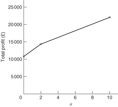
The previous two sections described how a lot of useful information could be derived concerning the effects on the optimal solution of changes in the coefficients of a linear programming model. Such information was, however, limited in value by the fact that (i) only one coefficient could be changed at a time and (ii) that coefficient could only be changed within certain ranges. Parametric programming is a convenient method of investigating the effects of more radical changes. It is beyond the scope of this book to describe how the method works. There is virtue, however, in describing how such investigations can be organized and presented to a computer package. Parametric programming is computationally quick and therefore provides a cheap means of determining how the optimal solution changes with alterations in objective and right-hand side coefficients. It is useful to illustrate the description again by means of a numerical example. We will again use the product mix model introduced in Section 1.2. In the last section we saw how the right-hand side coefficients could be varied individually within their permitted ranges. Suppose that instead we wished to investigate the possibility of increasing both grinding capacity and manpower simultaneously. Parametric programming on the right-hand side allows us to carry out such an investigation as long as the coefficients increase (or decrease) by constant relative amounts. For example, we could investigate the effect of employing an extra worker on assembly for each new grinding machine bought. Each increase of 96 hours per week in grinding capacity will therefore be accompanied by an increase of 48 hours per week in manpower capacity. If θ new grinding machines are bought, the right-hand side vector of coefficients would become
Parametric programming allows one to specify a change column such as
![]()
and limits within which θ can vary. The procedure will then allow θ to vary between these limits and calculate the value of the objective function at various intervals. For example, the parameter θ was allowed to vary between 0 (the original capacities) and 10 (when the new capacities become 1248, 192 and 864 respectively).
Such information can be very valuable in examining the effect of expansions or contractions in the availability of different resources. The result is well expressed graphically, as is done for the example we have just discussed in Figure 6.6.
Analogous to parametric programming on the right-hand side is parametric programming on the objective function. For example, in the product mix model, if we wished to increase the prices of all products by the same amount simultaneously, we would specify a change row:
![]()
A parameter θ would be allowed to vary between specified limits adding θ times this row to the row of objective coefficients. The effect on the optimal objective view would again be mapped out.
6.5 Presentation of the solutions
This chapter has described a lot of useful information which can be derived from linear programming models. It is often easy to lose sight of the difficulty which non-specialists may have in relating such information to the real life situation which has been modelled. Obscure presentation of information derived from a linear programming model can lead to complete rejection of the technique. Computer output is often obscure as a package program is designed to solve any model no matter what the application is. The output must obviously, therefore, relate to the mathematical aspects of the model. One way of overcoming the difficulty is for an intermediate person (possibly the model builder) to convert the computer output into a written report which can easily be understood. For models which are run frequently this can be a cumbersome and slow process. Many organizations have computer programs which read the solution output from the linear programming package and convert it into a form which relates to the application. Computer programs which do this are known as report writers. Clearly a report writer program must be related to the application. As a consequence such programs are usually purpose written for the type of model solved. Frequently they are written by the organization using the model rather than by the producer of the package. A high level language is usually used. It is necessary for the program to read the solution output from the package. With most packages it is quite easy to do this by getting the package to write its output on to a file. Many practitioners would argue in favour of such purpose-built report writers. There do, however, exist general purpose report writers which sometimes accompany particular packages. Sometimes these report writers can be used satisfactorily for the application required.
Report writers are often considered in conjunction with matrix generators which were discussed in Section 3.5. A matrix generator relates the input for a linear programming model to the practical problem while a report writer so relates the output.
In order to show the advantage of a report writer, the information is presented through a purpose-built report writer for the application. The output should be self-explanatory.
DATE: 1 JANUARY 1999