
Chapter 4
Structured linear programming models
4.1 Multiple plant, product and period models
The purpose of this section is to show how large linear programming (LP) models can arise through the combining of smaller models. Almost all very large models arise in this way. Such models prove to be more powerful as decision making tools than the submodels from which they are constructed. In order to illustrate how a multiplant model can arise in this way, we take a very small illustrative example.
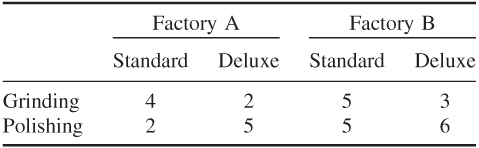
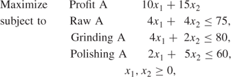
Factory A's Model
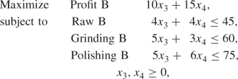
Factory B's Model
Optimal Solution to Factory A's Model
Optimal Solution to Factory B's Model
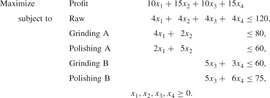
The Company Model
Optimal Solution to the Company Model
The above example is intended to show how a multiplant model can arise. It is a method of using LP to cope with allocation problems between plants as well as help with decision making within plants. The model that we built was a very simple example of a common sort of structure, which arises in multiplant models. This is known as a block angular structure. If we detach the coefficients in the company model and present the problem in a diagrammatic form, we obtain Figure 4.1.
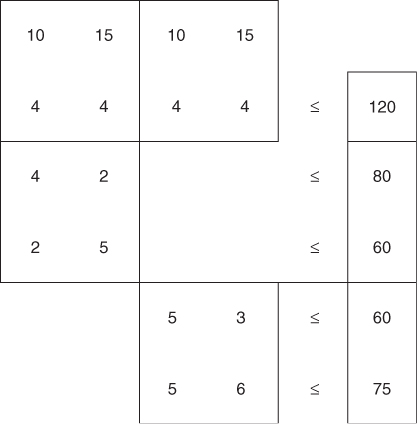
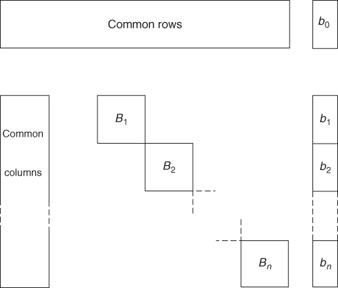
The first two rows are known as common rows. Obviously, one of the common rows will always be the objective row. The two diagonally placed blocks of coefficients are known as submodels. For a more general problem with a number of shared resources and n plants, we would obtain the general block angular structure shown in Figure 4.2.
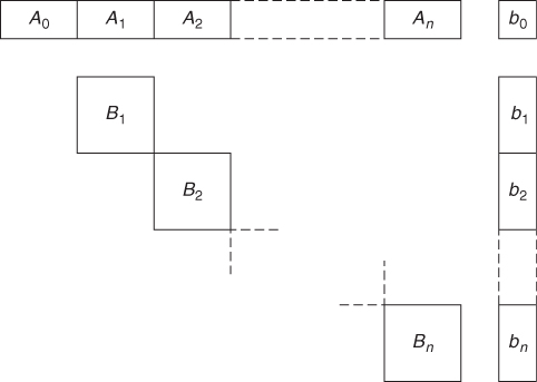
A0, A1, …, B1, B2, …, are blocks of coefficients. b0, b1, …, are columns of coefficients forming the right-hand side. The block A0 may or may not exist but is sometimes conveniently represented. A0, A1, …, represent the common rows. Common constraints in multiplant models usually involve allocating scarce resources (raw material, processing capacity, labour, etc.) across plants. They might sometimes represent transport relations between plants. For example, it might in certain circumstances be advantageous to transport the product of an intermediate process from one plant to another. The model could conveniently allow for this if extra variables were introduced into the plants in question to represent amounts transported. Suppose we simply wanted to allow for transport from plant 1 to plant 2. This would be accomplished by the constraint
where x1 is the quantity transported from 1 into 2 and x2 is the quantity transported into 2 from 1.
Apart from constraint (4.1), x1 would only be involved in constraints relating to the submodel for plant 1. Similarly, x2 would only be involved in constraints relating to plant 2. x1 (or x2 but not both) would probably be given cost coefficients in the objective function representing unit transport costs. Constraint (4.1) clearly gives another common row constraint.
Should a problem with a block angular structure have no common constraints, it should be obvious that optimizing it simply amounts to optimizing each subproblem with its appropriate portion of the objective. For our simple numerical example, if there had been no raw material constraint, we could have solved each factory's model separately and obtained an overall company optimum. In fact, as far as the company was concerned, it would have been perfectly acceptable to treat each factory as autonomous. Once we introduce common constraints, however, this will probably no longer be the case, as the small example demonstrated. The more common constraints there are, the more interconnected the separate plants must be. In Section 4.2, we discuss how a knowledge of the optimal solutions to the subproblems might be used to obtain an optimal solution to the total problem. This can be quite important computationally, as such structured problems can often be very large and take a long time to solve if treated as one large model. Common sense would suggest that the number of common rows would be a good measure of how close the optimal solution to the total problem was to the sum total of the optimal solutions to the subproblems. This is usually the case. For problems with only a few common rows, one might expect there to be virtue in taking account of the optimal solutions of the subproblems.
The block angular structure exhibited in Figure 4.2 does not arise only in multiplant models. Multi-product models arise quite frequently in blending problems. Suppose, for example, that the blending problem that we presented in Section 1.2 represented only one of a number of products (brands) that a company manufactured. If the different products used some of the same ingredients and processing capacity then it would be possible to take account of their limited supply through a structured model. The individual blending models such as those presented in Section 1.2 would be unable to help make rational allocations of such scarce shared resources between products. For example, in Figure 4.2, B1, B2, …, would represent the individual blending constraints for each product. These subproblems would contain variables such as xij representing the quantity of ingredient i in product j. If ingredient i was in limited supply, we would impose a common constraint:
4.2 ![]()
If ingredient i used αij units of a particular processing capacity in blending product j, we would have the common constraint:
4.3 ![]()
As with multiplant models, multi-product models almost always arise through combining existing submodels. The submodels can be used to help make certain operational decisions. By combining such submodels into multiple models, further decisions can be brought into the realm of LP.
Another way in which the block angular structure of Figure 4.2 arises is in multi-period models. Suppose that in our blending problem of Section 1.2, we wanted to determine not just how to blend in a particular month but also how to purchase each month with the possibility of storing for later use. It would then be necessary to distinguish between buying, using, and storing. For each ingredient, there would be three corresponding variables. These would be linked together by the relations:
These relations give equality constraints. The block angular structure of Figure 4.2 arises through these equality constraints providing common rows linking consecutive time periods. Each subproblem B1 consists of the original blending constraints involving only the ‘using’ variables. Such a multi-period model arises from the FOOD MANUFACTURE problem of Part 2. This problem is the blending problem of Section 1.2 taken over six months with different raw oil prices for different months. Full details of the formulation of this problem are given in Part 3.
In a multi-period model of the kind described above, each period need not necessarily be of the same duration. Some periods might be of a month, while later months might be aggregated together (with a corresponding increase in resources represented by right-hand side coefficients). It will, however, be very likely that B1, B2, …, in Figure 4.2 are the same submatrices representing the same blending constraints in each period. The corresponding rows and columns of these matrices will of course be distinguished by different names.
The way in which multi-period models should be used is important. Such a model is usually run with the first period relating to the present times and subsequent periods relating to the future. As a result, only the operating decisions suggested by the model for the present month are acted on. Operating decisions for future months will probably only be taken as provisional. After a further month (or the appropriate time period) has elapsed, the model will be rerun with updated data and the first period applying to the new present period. In this way, a multi-period model is in constant use as both an operating tool for the present and a provisional planning tool for the future.
A further point of importance in multi-period models concerns what happens at the end of the last time period in the model. If the stocks at the end of the last period, which occur in constraint (4.4), are included simply as variables, the optimal solution will almost always decide that they should be zero. From the point of view of the model, this would be sensible as it would be the minimum ‘cost’ or maximum ‘profit’ solution. In a practical situation, however, the model is unrealistic as operations will almost certainly continue beyond the end of the last period and stocks would probably not be allowed to run right down. One possible way out is to set the final stocks to constant values representing sensible final levels. It could be argued that the operating plans for the final period will be very provisional anyway and any inaccuracy that far ahead will not be serious. This is the suggestion that is made for dealing with both the multi-period FACTORY PLANNING and FOOD MANUFACTURE problems of Part 2. An alternative approach that is sometimes adopted is to ‘value’ the final stocks in some way, that is, give the appropriate variables positive ‘profits’ in a maximization model or negative ‘costs’ in a minimization model. In effect, such a valuation would cause the optimal solution to suggest producing final stocks to sell if it appeared profitable. Although the organization might never consider the possibility of selling off final stocks, the fact that they had been given realistic valuations would cause them to come out at sensible levels.
A description of a highly structured model that is potentially multi-period, multi-product and multiplant is given by Williams and Redwood (1974).
Another type of structure that often arises in multi-period models is the staircase structure. This is illustrated in Figure 4.3.
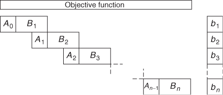
In fact, a staircase structure such as this could be converted into a block angular structure. If alternate ‘steps’ such as (A0, B1), (A2, B3) were treated as subproblem constraints and the intermediate ‘steps’ as common rows, we would have a block angular structure. The block angular multi-period model, which was described above, could also easily be rearranged into a staircase structure.
Another structure that sometimes arises, although less commonly than block angular and staircase structures, is shown in Figure 4.4.
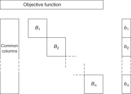
In this type of model, the subproblems are connected by common columns rather than rows. Such a structure is the dual to the block angular structure (the dual is defined in Section 6.2).
The method of Benders (1962) is applicable to solving these types of model (even if they are not integer programmes). A way in which this type of structure arises is given in the next section.
4.2 Stochastic programmes
Stochastic programmes are a special type of LP model. Although the title ‘Stochastic Programming’ is sometimes used, it can convey the misleading impression that this is another technique. A stochastic programme is a type of LP, which models uncertainty in a particular way. Stochastic programming is a special case of robust optimization. In many practical situations, the data in a resultant LP model is not known with certainty. This may be for a number of reasons. One is an inability to obtain totally accurate data. Another is that the model is time staged (discussed in Section 4.1) where certain events, which need to be modelled, have not yet occurred. Robust optimization encompasses both these situations, even when we cannot quantify the uncertainty or associated risks. It is concerned with obtaining solutions that remain reasonably stable in the face of the uncertainty, whether it can be quantified or not. The use of sensitivity analysis, which is discussed in Section 6.3, gives information on how a solution changes with uncertainty in the data. This is a rather limited analysis that can be misleading in some circumstances, see Kall and Wallace (1994). A totally risk-averse approach might be to seek a maximin solution (as discussed in Section 3.2) in order to make the worst possible result (however unlikely) as little bad as possible. Often, however, this extreme approach is excessively ‘conservative’. A very good discussion of robust optimization is given by Greenberg and Morrison (2008).
In this section, we confine ourselves to situations where the uncertainty can be quantified. One way of modelling some such situations is by chance constraints as discussed in Section 3.3. We will confine ourselves, here, to modelling situations where some decisions (stage 1) have to be made before other information becomes available. The result of the stage 1 decisions and the subsequent availability of extra information allow stage 2 decisions to be made. Unfortunately, the relative merits of the stage 1 decisions depend on this uncertain information and the resultant stage 2 decisions. For example, it may be necessary to decide production (stage 1) before the demand (uncertain) is known. Then as a result of the production decisions and the subsequent actual demand, stage 2 decisions must be made regarding selling any excess production at a lower price or extra production to make up a shortfall at a higher cost.
If it is realistic to consider the uncertain information as taking one of a (small) finite number of possible values with known probabilities (a discrete probability distribution) then a set of distinct stage 2 variables may be introduced to correspond to each uncertain value. The objective becomes one of minimizing expected cost. This model then becomes a linear program.
For example, suppose that the production decisions are represented by stage 1 variables x1, x2, …, xn. The excess production or shortfall is represented by stage 2 variables y1, y2, …, yn, z1, z2, …, zn. These stage 2 variables will be replicated m times according to each of the possible demand levels ![]() . This gives a model of the form:
. This gives a model of the form:
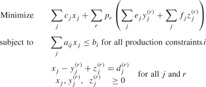
where pr are given probabilities and cj, ej and fj are production, excess production, and shortfall costs, respectively.
It is important to realize how such a model might be used. Initial decisions would be made as a result of stage 1 variables. Only the values of those stage 2 variables would ultimately be used, which corresponded to the subsequent value of the uncertain information.
Also, it is important to realize the extra information that is incorporated in such a model. While a ‘conventional’ model may contain future data in the form of a single ‘point’ estimate, a stochastic model represents such data by a series of estimates, weighted by probabilities. The result may be a ‘solution’ that is not as ‘good’ as the conventional model, in terms of optimal objective, but that is more likely to be realistic, to be realizable, and to reduce risk. Another way of viewing such models is one of ‘keeping one's options open’, that is, not ‘putting all one's eggs in one basket’.
The coefficients of the xj variables, above, form the common columns of the LP model, while the variables ![]() and
and ![]() each appear in only the rth block of the model. The combination of this structure with the block angular structure sometimes occurs giving models of the form shown in Figure 4.5.
each appear in only the rth block of the model. The combination of this structure with the block angular structure sometimes occurs giving models of the form shown in Figure 4.5.
An example of the use of a stochastic program is YIELD MANAGEMENT (selling airline tickets), which is given in Sections 12.24, 13.24 and 14.24.
References to stochastic programming are Dempster (1980), Kall and Wallace (1994) and Greenberg and Morrison (2008). Stochastic programmes can become very large because of the multiplicity of scenarios resulting from successive periods, that is, from each scenario in the second stage, there will be a number of scenarios into the third stage, etc. The resultant tree of scenarios into the future rapidly becomes very large. The largest LP ever built and solved (to the author's belief) is a stochastic program due to Gondzio and Grothey (2006). It has 353 million constraints and 1010 million variables.
4.3 Decomposing a large model
Common sense suggests that the optimal solution to a structured model should bear some relation to the optimal solutions to the submodels from which it is constructed. This is usually the case and there may, therefore, be virtue in devising computational procedures to exploit this, particularly in view of the large size of many structured models. Ways of solving a structured model by way of solutions to the subproblems form the subject of decomposition. It is sometimes mistakenly thought that decomposition is the actual act of splitting a model up into submodels. Although computational procedures have been devised for doing this, decomposition concerns the solution process on a structure that is usually already known to the modeler.
The importance of decomposition is not only computational but also economic. A decomposition procedure applies to a mathematical model of a structured practical problem. If the structured model arises by way of a structured organization (such as a multiplant model), the decomposition procedure mirrors a method of decentralized planning. It is for this reason that decomposition is discussed in a book on model building. The subject is best considered through this analogy with decentralized planning.
We will again consider the small illustrative problem of Section 4.1, which gave rise to the following multiplant model:
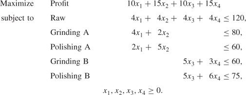
It was seen that splitting the 120 kg of raw between A and B in the ratio 75 : 45 led to a non-optimal overall solution. The optimal overall solution showed that this ratio should be 70 : 50. Unfortunately, we had to solve the total model in order to find this optimal split. If we had a method of predetermining this optimal split, we would be able to solve the individual models for factories A and B and combine the solutions to give an optimal solution for the total model. For a general block angular model, as illustrated in Figure 4.2, we would need to find optimal splits in all the right-hand side coefficients in b0 for the common rows. Algorithms for the decomposition of a block angular structure based on this principle do exist. Such methods are known as decomposition by allocation. One such algorithm is the method of Rosen (1964).
An alternative approach is decomposition by pricing. In a block angular structure, such as our small example above where common rows represent constraints on raw material availability, we could try to seek valuations for the limited raw material. These valuations could be used as internal prices to be charged to the submodels. If accurate valuations could be obtained, we might hope to get each submodel optimizing to the overall benefit of the total model. One such approach to this is the Dantzig–Wolfe decomposition algorithm. A full description of the algorithm is given in Dantzig (1963). We provide a less rigorous description here paying attention to the economic analogy with decentralized planning.
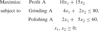
To illustrate the method, we again use the small two-factory example. If it were not for the raw material being in limited supply, we would have the following submodels for A and B:
These submodels should not be confused with the submodels for the same problem in Section 4.1. The raw availability constraints were included in both submodels with a suitable allocation of raw material between them. Here, we are not including such constraints. Instead, an attempt is made to find a suitable ‘internal price’ for raw and to incorporate this into the submodels. Suppose that raw were to be internally priced at £p per kilogram. The objective functions for the above submodels would then become
and
In effect, we have taken multiples of p times the raw material availability constraints and subtracted them from the objectives. If p is set too low, we might find that the combined solutions to the submodels use more raw than is available in which case p should be increased. For example, if p is taken as zero (there is no internal charge for raw), we obtain the following optimal solutions:
Factory A's Optimal Solution with Raw Valued at 0
Factory B's Optimal Solution with Raw Valued at 0
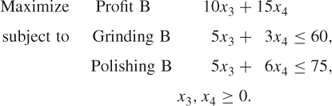
These solutions are clearly unacceptable to the company as a whole, as they demand 140 kg of raw, which is more than the 120 kg available. We, therefore seek some way of estimating a more realistic value for the internal price p. Whatever the value of p, A and B will have optimal solutions that are vertex solutions of the submodels presented above. As these models only involve two variables each, they can be represented graphically. This is shown in Figures 4.6 and 4.7.
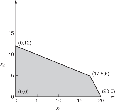
With the value of zero for p, we can easily verify the optimal solutions above for A and B as being (17.5, 5) in Figure 4.6 and (0, 12.5) in Figure 4.7.
Any feasible solution to the total problem must clearly be feasible with respect to both subproblems (as well as additionally satisfying raw material availability limitation). The values of x1 and x2 in any feasible solution to the total problem must, therefore, be a convex linear combination of the vertices of the feasible region shown in Figure 4.6, that is,
λ11, λ12, λ13, and λ14 are ‘weights’ attached to the vertices. They must be non-negative and satisfy the convexity condition:
The vector Equation (4.7) is a way of relating x1 and x2 to a new set of variables λij by the following two equations:
4.10 ![]()
A similar argument can be applied to the second subproblem represented in Figure 4.7. This allows x3 and x4 to be related to yet more variables λ21, λ22, λ23, and λ24 by the following equations:
4.11 ![]()
λ2j are ‘weights’ for vertices in the second subproblem while λ2j are ‘weights’ in the first subproblem.
It is worth pointing out that what we are really doing is giving modal formulations, as described in Section 3.4, for each subproblem.
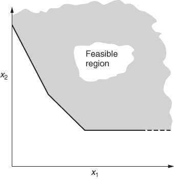
A slight complication arises if the feasible regions of some of the submodels are ‘open’, for example, we have the situation shown in Figure 4.8. This complication is easily dealt with and fully explained in Dantzig (1963).
We can use Equations (4.9)–(4.12) to substitute for x1, x2, x3 and x4 in the objective and single common constraint raw of our total model. The grinding and polishing constraints of the two subproblems will be satisfied so long as the λij are non-negative and satisfy the convexity constraints, Equations (4.8) and (4.13). In this way, our multiplant model can be re-expressed as
The above model is known as the master model. It can be interpreted as a model to find the ‘optimum mix’ of vertex solutions of each of the submodels. For any internal price p, which is charged to A and B, they will each produce vertex solutions. Such vertex solutions give rise to what are known as proposals, as they represent ‘proposed’ solutions from the submodels, given the provisional internal price p for raw. The proposals are the columns of coefficients in the master model corresponding to a particular vertex of a submodel. For example, the proposal from the third vertex of the first subproblem is the column

This proposal is given a weight of λ13 in the master model. The role of the master model is to choose the best combination of all the proposals that have been obtained.
The master model would generally have far fewer constraints than the original model. There will be the same number of common rows as in the total model. Each submodel will, however, have been condensed down into a single convexity constraint such as conv 1 in the example above. Unfortunately, the saving-in constraints will generally be more than offset by a vast expansion in the number of variables. We will have a λij variable for each vertex of each submodel. This could be an astronomical number in a realistic problem. In practice, the great majority of proposals corresponding to these variables will be zero in an optimal solution. For a master model with a comparatively small number of constraints, but a very large number of variables, the great majority of variables will never enter a solution. We therefore resort to a practice that is used quite widely in mathematical programming. Columns are generated in the course of optimization. A column (proposal) is added to the master model only when it seems worthwhile. This is an example of column generation, which is discussed in Section 9.6. We therefore deal only with a subset of the possible proposals. Such a truncated model is known as a restricted master model. Proposals are added to (and sometimes deleted from) the restricted master model in the course of optimization. In general, only a very small number of the potential proposals will ever be generated and added to the restricted master problem.
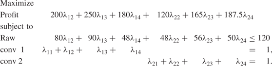
In order to describe how we proceed, we will consider our small multiplant model. Instead of using the master model, which we were fortunate enough to be able to obtain from geometrical considerations in so small an example, we will work with a restricted master problem. To start with we will take only the proposals corresponding to λ11 and λ13 from submodel A and λ21 and λ24 from submodel B. This choice is largely arbitrary. How it is made is not important to our discussion. In practice, a number of ‘good’ proposals from each submodel would be used to make up the first version of the restricted master model in order to have a reasonably realistic model with some substance. Our first restricted master model is therefore
When this model is optimized, we can obtain a ‘valuation’ for the raw material. This valuation is the marginal value of the raw constraint in the optimal solution. Such marginal values for constraints are sometimes known as shadow prices. They are discussed much more fully together with their economic interpretation in Section 6.2. In fact, the marginal value associated with a constraint such as raw is the rate at which the optimal profit would increase for small (‘marginal’) increases in the right-hand side coefficient. It is sufficient for our purpose here simply to remark that such valuations for constraints are possible. With any package programs, these valuations (shadow prices) are presented with the optimal solution.
If our first restricted master model is optimized, the shadow price on the raw constraint turns out to be £2.78. This can be taken as value p and used as an internal price, which factories A and B are charged for each kilogram of raw that they wish to use. When A is charged, this internal price it will reform its objective function to take account of the new charge. The new objective function comes from the expression (4.5) taking p as £2.78. This gives
4.14 ![]()
If this objective is used with the constraints of the submodel for A, we obtain the solution
![]()
This clearly corresponds to the vertex (0, 12) in Figure 4.6. The proposal corresponding to this is the column for λ14. This is easily calculated to be

A new variable (λ14 but with a different name) is therefore added to the restricted master problem with this column of coefficients. This new proposal represents factory A's new provisional production plan given the new internal charge for raw.
Our attention is now turned to factory B. When they are charged £2.78 per kilogram for raw, the expression (4.6) gives their objective function as
4.15 ![]()
When this objective is optimized with the constraints of the submodel for factory B, we obtain the solution
![]()
We have the vertex (0, 12.5) in Figure 4.7. The proposal corresponding to this is the column for λ24. This proposal has already been included in our first restricted master model. We, therefore, conclude that even if factory B is charged at the suggested rate of £2.78 per kilogram for raw, they would not suggest a new proposal (provisional production plan).
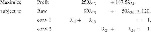
Having added only the proposal corresponding to λ14 to our restricted master model, it now becomes
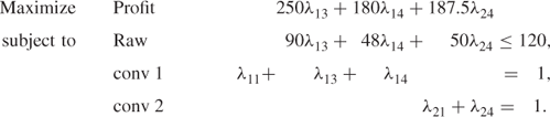
Optimizing this model, the shadow price on raw turns out to be £1.67. We see that our previous valuation of £2.78 appears to have been an over estimate.
The cycle is now repeated and each factory is internally charged £1.67 per kilogram for raw. This gives the following new objectives for A and B:
When the objective (4.16) is used with the constraints of the submodel for factory A, the optimal solution obtained is
![]()
This is the vertex (17.5, 5) in Figure 4.6 and gives the proposal corresponding to λ13. As this proposal has already been incorporated in the restricted master problem, factory A has no new proposal to offer as a result of the revised internal charge of £1.67 per kilogram for raw.
Factory B optimizes objective (4.17) subject to the constraints of its submodel. This results in the solution:
![]()
This is the vertex (0, 12.5) of Figure 4.7, which results in the proposal corresponding to λ24. As this proposal is already present in the restricted master model, factory B also has no further useful proposal to add as a result of the revised charge for raw.
We therefore conclude that factories A and B have submitted all the useful proposals that they can. The optimal solution to the latest version of the restricted master model gives the proportions in which these proposals should be used. For our example, the optimal solution to this restricted master model is
![]()
This enables us to calculate the optimal values for x1, x2, x3, and x4 by considering the vertex solutions of the submodels corresponding to λ13 and λ14, and λ24. We obtain
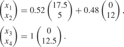
This gives us the optimal solution to the total model,
![]()
giving an objective value of £404.15.
Notice, however, that we have obtained the optimal solution to the total model without solving it directly. Instead, we have dealt with what would generally be much smaller models. The two types of model we have used are the submodels and the restricted master model. We further discuss the significance of these models below.
4.3.1 The submodels
These contain the details relevant to the individual subproblems. For a multiplant model such as that used in our example, the coefficients in the constraints concern only the particular factory, that is, grinding and polishing times and capacities in each factory.
4.3.2 The restricted master model
This is an overall model for the whole organization but, unlike the total model, it contains none of the technological detail relating to the individual subproblems. Such detail is left to the submodels. Instead, the constraints for each subproblem are accounted for by a simple convexity constraint. In our example, we had the constraints for factories A and B reducing to convexity constraints conv 1 and conv 2, respectively. On the other hand, the restricted master model does contain the common rows in full, as its main purpose is to determine suitable valuations for the resources represented by these common rows.
By means of interactions between the submodels and the restricted master model, it is possible eventually to obtain the optimal solution to the (usually much larger) total model without ever building and solving it directly. The process that we describe here is diagrammatically represented in Figure 4.9.
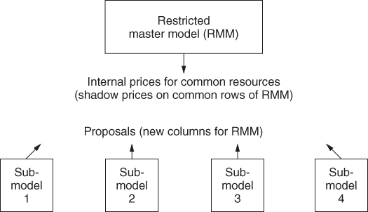
There is considerable attraction in such a scheme, as it is never necessary to build, solve, and maintain the often huge total model, which would result from a large structured organization. In a multiplant organization, the individual plants would probably be geographically separated. This would make the avoidance of including all their technological details in one central model desirable. Each plant might well build and maintain their own model inside their own plant and solve it on their own computer. The head office could maintain a restricted master model on another computer, which would be linked to the computers in the individual plants. Each model could then be run independently but could supply the vital information of proposals and internal prices to the other models. It would then be possible to use a system automatically to obtain an overall optimal solution for the organization.
Decomposition has interest for economists, as it clearly represents a system of decentralized planning. The existence of decomposition algorithms such as the Dantzig–Wolfe algorithm demonstrates that it is possible to devise a method of decentralized planning, which achieves an optimal solution for an organization considered as a whole. This is done by allowing the suborganizations to decide their own optimal policies, given limited control from the centre. In the case of the Dantzig–Wolfe algorithm, this control takes the form of internal prices. For other methods, it may take the form of allocations. An informal version of such procedures takes place in many organizations. A discussion of a large number of decomposition algorithms and their relation to decentralized planning in real life is given by Atkins (1974).
Decomposition algorithms are also of considerable computational interest, as they offer a possibility of avoiding the large amount of time needed to solve large models should those models be structured. Unfortunately, decomposition has only met with limited computational success. The most widely used algorithm is the Dantzig–Wolfe algorithm that applies to block angular structured models. There are many circumstances, however, in which it is more efficient to solve the total model rather than to use decomposition. The main advice to someone building a structured model should not be to attempt decomposition on other than an experimental basis. As experience and knowledge grow, decomposition may well become a more reliable tool, but at present, the computational experience with such methods has been disappointing. If a model is to be used very frequently, experimenting with decomposition might be considered worthwhile. The larger the model and the smaller the proportion of common rows (for block angular structures), the more valuable this is likely to be. Sometimes, other aspects of the structure can be exploited to advantage. An example of this is described by Williams and Redwood (1974). Computational experiences using Dantzig–Wolfe decomposition are given by Beale et al. (1965) and Ho and Loute (1981). A very full description of the computational side of decomposition is given by Lasdon (1970). Finally, decomposition may commend itself for the purely organizational considerations resulting from the desirability of decentralized planning.
The use of communication networks for linking computers together makes it possible to implement a decomposition algorithm splitting the models between different computers, e.g. the master model in the head office and the submodels at individual plants. This idea has not, to the author's knowledge, yet been tried.