
Chapter 12
The problems
There is no significance in the order in which the following 29 problems are presented. Some are easy to formulate and present no computational difficulties in solution, while others are more difficult in either or both of these respects. Some can be solved with linear programming; others require integer programming or separable programming.
It is suggested that readers attempt to formulate those problems that interest them before consulting the formulations and solutions proposed in Parts III and IV. A computer package may be used on the model, or an intuitive (heuristic) approach to some of the problems may be attempted, using original methods of the reader's own choosing; answers can then be compared with the optimal solutions given in Part IV.
Readers wishing to follow the recommended course of solving the models using a computer package are strongly advised to use a matrix generator/language, as discussed in Sections 3.5 and 4.3. This will enable them to concentrate on the structure of the model as well as facilitating error detection and greatly reducing data preparation.
12.1 Food manufacture 1
A food is manufactured by refining raw oils and blending them together. The raw oils are of two categories:
| Vegetable oils | VEG 1 VEG 2 |
| Non-vegetable oils | OIL 1 OIL 2 OIL 3 |
Each oil may be purchased for immediate delivery (January) or bought on the futures market for delivery in a subsequent month. Prices at present and in the futures market are given below in (£/ton):

The final product sells at £150 per ton.
Vegetable oils and non-vegetable oils require different production lines for refining. In any month, it is not possible to refine more than 200 tons of vegetable oils and more than 250 tons of non-vegetable oils. There is no loss of weight in the refining process, and the cost of refining may be ignored.
It is possible to store up to 1000 tons of each raw oil for use later. The cost of storage for vegetable and non-vegetable oil is £5 per ton per month. The final product cannot be stored, nor can refined oils be stored.
There is a technological restriction of hardness on the final product. In the units in which hardness is measured, this must lie between 3 and 6. It is assumed that hardness blends linearly and that the hardnesses of the raw oils are
| VEG 1 | 8.8 |
| VEG 2 | 6.1 |
| OIL 1 | 2.0 |
| OIL 2 | 4.2 |
| OIL 3 | 5.0 |
What buying and manufacturing policy should the company pursue in order to maximise profit?
At present, there are 500 tons of each type of raw oil in storage. It is required that these stocks will also exist at the end of June.
This problem, and the subsequent problem, is based on a larger model built for the margarine producer Van den Bergs and Jurgens and discussed in Williams and Redwood (1974).
12.2 Food manufacture 2
It is wished to impose the following extra conditions on the food manufacture problem:
Extend the food manufacture model to encompass these restrictions and find the new optimal solution.
12.3 Factory planning 1
An engineering factory makes seven products (PROD 1 to PROD 7) on the following machines: four grinders, two vertical drills, three horizontal drills, one borer and one planer. Each product yields a certain contribution to profit (defined as £/unit selling price minus cost of raw materials). These quantities (in £/unit) together with the unit production times (hours) required on each process are given below. A dash indicates that a product does not require a process.
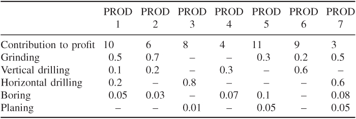
In the present month (January) and the five subsequent months, certain machines will be down for maintenance. These machines will be as follows:
| January | 1 Grinder |
| February | 2 Horizontal drills |
| March | 1 Borer |
| April | 1 Vertical drill |
| May | 1 Grinder and 1 Vertical drill |
| June | 1 Planer and 1 Horizontal drill |
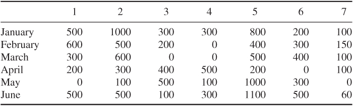
There are marketing limitations on each product in each month. These are given in the following table:
It is possible to store up to 100 of each product at a time at a cost of £0.5 per unit per month. There are no stocks at present, but it is desired to have a stock of 50 of each type of product at the end of June.
The factory works a six days a week with two shifts of 8 h each day.
No sequencing problems need to be considered.
When and what should the factory make in order to maximise the total profit? Recommend any price increases and the value of acquiring any new machines.
N.B. It may be assumed that each month consists of only 24 working days.
This problem, and the subsequent problem, is based on a larger model built for the Cornish engineering company of Holman Brothers (which no longer exists).
12.4 Factory planning 2
Instead of stipulating when each machine is down for maintenance in the factory planning problem, it is desired to find the best month for each machine to be down.
Each machine must be down for maintenance in one month of the six apart from the grinding machines, only two of which need be down in any six months.
Extend the model to allow it to make these extra decisions. How much is the extra flexibility of allowing down times to be chosen worth?
12.5 Manpower planning
A company is undergoing a number of changes that will affect its manpower requirements in future years. Owing to the installation of new machinery, fewer unskilled but more skilled and semi-skilled workers will be required. In addition to this, a downturn in trade is expected in the next year, which will reduce the need for workers in all categories. The estimated manpower requirements for the next three years are as follows:
The company wishes to decide its policy with regard to the following over the next three years:
There is a natural wastage of labour. A fairly large number of workers leave during their first year. After this, the rate is much smaller. Taking this into account, the wastage rates can be taken as follows: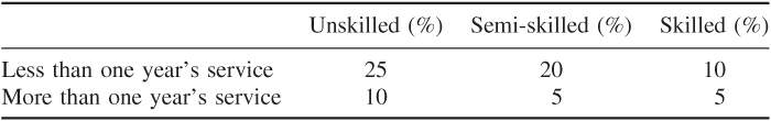
There has been no recent recruitment and all workers in the current labour force have been employed for more than one year.
12.5.1 Recruitment
It is possible to recruit a limited number of workers from outside. In any one year, the numbers that can be recruited in each category are as follows:
| Unskilled | Semi-skilled | Skilled |
| 500 | 800 | 500 |
12.5.2 Retraining
It is possible to retrain up to 200 unskilled workers per year to make them semi-skilled. This costs £400 per worker. The retraining of semi-skilled workers to make them skilled is limited to no more than one quarter of the skilled labour force at the time as some training is done on the job. Retraining a semi-skilled worker in this way costs £500.
Downgrading of workers to a lower skill is possible but 50% of such workers leave, although it costs the company nothing. (This wastage is additional to the ‘natural wastage’ described above).
12.5.3 Redundancy
The redundancy payment to an unskilled worker is £200 and to a semi-skilled or skilled worker is £500.
12.5.4 Overmanning
It is possible to employ up to 150 more workers over the whole company than are needed, but the extra costs per employee per year are as follows:
| Unskilled | Semi-skilled | Skilled |
| £1500 | £2000 | £3000 |
12.5.5 Short-time working
Up to 50 workers in each category of skill can be put on short-time working. The cost of this (per employee per year) is as follows:
| Unskilled | Semi-skilled | Skilled |
| £500 | £400 | £400 |
An employee on short-time working meets the production requirements of half a full-time employee.
The company's declared objective is to minimise redundancy. How should they operate in order to do this?
If their policy were to minimise costs, how much extra would this save? Deduce the cost of saving each type of job each year.
12.6 Refinery optimisation
An oil refinery purchases two crude oils (crude 1 and crude 2). These crude oils are put through four processes: distillation, reforming, cracking and blending, to produce petrols and fuels that are sold.
12.6.1 Distillation
Distillation separates each crude oil into fractions known as light naphtha, medium naphtha, heavy naphtha, light oil, heavy oil and residuum according to their boiling points. Light, medium and heavy naphthas have octane numbers of 90, 80 and 70, respectively. The fractions into which one barrel of each type of crude splits are given in the following table: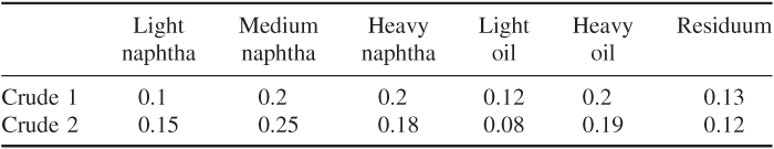
N.B. There is a small amount of wastage in distillation.
12.6.2 Reforming
The naphthas can be used immediately for blending into different grades of petrol or can go through a process known as reforming. Reforming produces a product known as reformed gasoline with an octane number of 115. The yields of reformed gasoline from each barrel of the different naphthas are given as follows:
12.6.3 Cracking
The oils (light and heavy) can either be used directly for blending into jet fuel or fuel oil or be put through a process known as catalytic cracking. The catalytic cracker produces cracked oil and cracked gasoline. Cracked gasoline has an octane number of 105.
Cracked oil is used for blending fuel oil and jet fuel; cracked gasoline is used for blending petrol.
Residuum can be used for either producing lube-oil or blending into jet fuel and fuel oil:
12.6.4 Blending
12.6.4.1 Petrols (motor fuel)
There are two sorts of petrol, regular and premium, obtained by blending the naphtha, reformed gasoline and cracked gasoline. The only stipulations concerning them are that regular must have an octane number of at least 84 and that premium must have an octane number of at least 94. It is assumed that octane numbers blend linearly by volume.
12.6.4.2 Jet fuel
The stipulation concerning jet fuel is that its vapour pressure must not exceed 1 kg cm2. The vapour pressures for light, heavy, cracked oils and residuum are 1.0, 0.6, 1.5 and 0.05 kg cm2, respectively. It may again be assumed that vapour pressures blend linearly by volume.
12.6.4.3 Fuel oil
To produce fuel oil, light oil, cracked oil, heavy oil and residuum must be blended in the ratio 10:4:3:1.
There are availability and capacity limitations on the quantities and processes used as follows:
The profit contributions from the sale of the final products are (in pence per barrel) as follows:
| Premium petrol | 700 |
| Regular petrol | 600 |
| Jet fuel | 400 |
| Fuel oil | 350 |
| Lube-oil | 150 |
How should the operations of the refinery be planned in order to maximise total profit?
12.7 Mining
A mining company is going to continue operating in a certain area for the next five years. There are four mines in this area, but it can operate at most three in any one year. Although a mine may not operate in a certain year, it is still necessary to keep it ‘open’, in the sense that royalties are payable, if it be operated in a future year. Clearly, if a mine is not going to be worked again, it can be permanently closed down and no more royalties need be paid. The yearly royalties payable on each mine kept ‘open’ are as follows:
| Mine 1 | £5 million |
| Mine 2 | £4 million |
| Mine 3 | £4 million |
| Mine 4 | £5 million |
There is an upper limit to the amount of ore, which can be extracted from each mine in a year. These upper limits are as follows:
| Mine 1 | 2 × 10⁶ tons |
| Mine 2 | 2.5 × 10⁶ tons |
| Mine 3 | 1.3 × 10⁶ tons |
| Mine 4 | 3 × 10⁶ tons |
The ore from the different mines is of varying quality. This quality is measured on a scale so that blending ores together results in a linear combination of the quality measurements, for example, if equal quantities of two ores were combined, the resultant ore would have a quality measurement half way between that of the ingredient ores. Measured in these units the qualities of the ores from the mines are given as follows:
| Mine 1 | 1.0 |
| Mine 2 | 0.7 |
| Mine 3 | 1.5 |
| Mine 4 | 0.5 |
In each year, it is necessary to combine the total outputs from each mine to produce a blended ore of exactly some stipulated quality. For each year, these qualities are as follows:
| Year 1 | 0.9 |
| Year 2 | 0.8 |
| Year 3 | 1.2 |
| Year 4 | 0.6 |
| Year 5 | 1.0 |
The final blended ore sells for £10 ton each year. Revenue and expenditure for future years must be discounted at a rate of 10% per annum.
Which mines should be operated each year and how much should they produce?
This problem is based on a larger one arising in deciding which pits to work in the firm of English China Clays. In that problem (in the 1970s), it was wished to work up to 4 mines out of 20 in each year. The model proved very difficult to solve.
12.8 Farm planning
A farmer wishes to plan production on his 200 acre farm over the next five years.
At present, he has a herd of 120 cows. This is made up of 20 heifers and 100 milk-producing cows. Each heifer needs 2/3 acre to support it and each dairy cow 1 acre. A dairy cow produces an average of 1.1 calves per year. Half of these calves will be bullocks, which are sold almost immediately for an average of £30 each. The remaining heifers can be either sold almost immediately for £40 or reared to become milk-producing cows at two years old. It is intended that all dairy cows be sold at 12 years old for an average of £120 each, although there will probably be an annual loss of 5% per year among heifers and 2% among dairy cows. At present, there are 10 cows each aged from newborn to 11 years old. The decision of how many heifers to sell in the current year has already been taken and implemented.
The milk from a cow yields an annual revenue of £370. A maximum of 130 cows can be housed at the present time. To provide accommodation for each cow beyond this number will entail a capital outlay of £200 per cow. Each milk-producing cow requires 0.6 tons of grain and 0.7 tons of sugar beet per year. Grain and sugar beet can both be grown on the farm. Each acre yields 1.5 tons of sugar beet. Only 80 acres are suitable for growing grain. They can be divided into four groups whose yields are as follows:
| Group 1 | 20 acres | 1.1 tons per acre |
| Group 2 | 30 acres | 0.9 tons per acre |
| Group 3 | 20 acres | 0.8 tons per acre |
| Group 4 | 10 acres | 0.65 tons per acre |
Grain can be bought for £90 per ton and sold for £75 per ton. Sugar beet can be bought for £70 per ton and sold for £58 per ton.
The labour requirements are as follows:
| Each heifer | 10 h per year |
| Each milk-producing cow | 42 h per year |
| Each acre put to grain | 4 h per year |
| Each acre put to sugar beet | 14 h per year |
Other costs are as follows:
| Each heifer | £50 per year |
| Each milk-producing cow | £100 per year |
| Each acre put to grain | £15 per year |
| Each acre put to sugar beet | £10 per year |
Labour costs for the farm are at present £4000 per year and provide 5500 h labour. Any labour needed above this will cost £1.20 per hour.
How should the farmer operate over the next five years to maximise profit? Any capital expenditure would be financed by a 10-year loan at 15% annual interest. The interest and capital repayment would be paid in 10 equally sized yearly instalments. In no year can the cash flow be negative. Finally, the farmer would neither wish to reduce the total number of dairy cows at the end of the five-year period by more than 50% nor wish to increase the number by more than 75%.
12.9 Economic planning
An economy consists of three industries: coal, steel and transport. Each unit produced by one of the industries (a unit will be taken as £1's worth of value of production) requires inputs from possibly its own industry as well as other industries. The required inputs as well as the manpower requirements (also measured in £) are given in Table 12.1. There is a time lag in the economy so that the output in year t + 1 requires an input in year t.
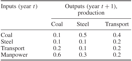
Output from an industry may also be used to build productive capacity for itself or other industries in future years. The inputs required to give unit increases (capacity for £1's worth of extra production) in productive capacity are given in Table 12.2. Input from an industry in year t results in a (permanent) increase in productive capacity in year t + 2.

Stocks of goods may be held from year to year. At present (year 0), the stocks and productive capacities (per year) are given in Table 12.3 (in £m). There is a limited yearly manpower capacity of £470 m.
| Year 0 | ||
| Stocks | Productive capacity | |
| Coal | 150 | 300 |
| Steel | 80 | 350 |
| Transport | 100 | 280 |
It is wished to investigate different possible growth patterns for the economy over the next five years. In particular, it is desirable to know the growth patterns that would result from pursuing the following objectives:
12.10 Decentralisation
A large company wishes to move some of its departments out of London. There are benefits to be derived from doing this (cheaper housing, government incentives, easier recruitment, etc.), which have been costed. Also, however, there will be greater costs of communication between departments. These have also been costed for all possible locations of each department.
Where should each department be located so as to minimise overall yearly cost?
The company comprises five departments (A, B, C, D and E). The possible cities for relocation are Bristol and Brighton, or a department may be kept in London. None of these cities (including London) may be the location for more than three of the departments.
Benefits to be derived from each relocation are given (in thousands of pounds per year) as follows: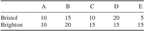
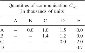
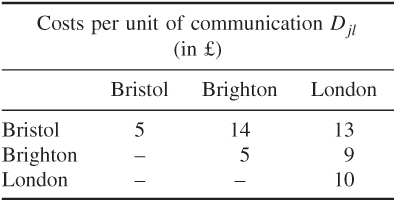
Communication costs are of the form CikDjl, where Cik is the quantity of communication between departments i and k per year and Djl is the cost per unit of communication between cities j and l. Cik and Djl are given by the following tables:
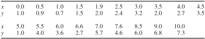
12.11 Curve fitting
A quantity y is known to depend on another quantity x. A set of corresponding values has been collected for x and y and is presented in Table 12.4.
12.12 Logical design
Logical circuits have a given number of inputs and one output. Impulses may be applied to the inputs of a given logical circuit, and it will respond by giving either an output (signal 1) or no output (signal 0). The input impulses are of the same kind as the outputs, that is, 1 (positive input) or 0 (no input).
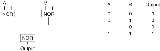
In this example, a logical circuit is to be built up of NOR gates. A NOR gate is a device with two inputs and one output. It has the property that there is positive output (signal 1) if and only if neither input is positive, that is, both inputs have the value 0. By connecting such gates together with outputs from one gate possibly being inputs into another gate, it is possible to construct a circuit to perform any desired logical function. For example, the circuit illustrated in Figure 12.1 will respond to the inputs A and B in the way indicated by the truth table.
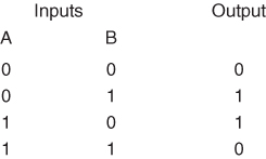
The problem here is to construct a circuit using the minimum number of NOR gates that will perform the logical function specified by the truth table in Figure 12.2. This problem, together with further references to it, is discussed in Williams (1974).
‘Fan-in’ and ‘fan-out’ are not permitted. That is, more than one output from a NOR gate cannot lead into one input nor can one output lead into more than one input.
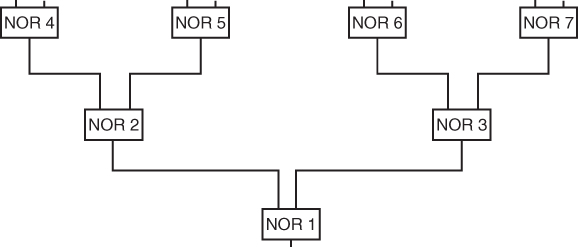
It may be assumed throughout that the optimal design is a ‘subnet’ of the ‘maximal’ net shown in Figure 12.3.
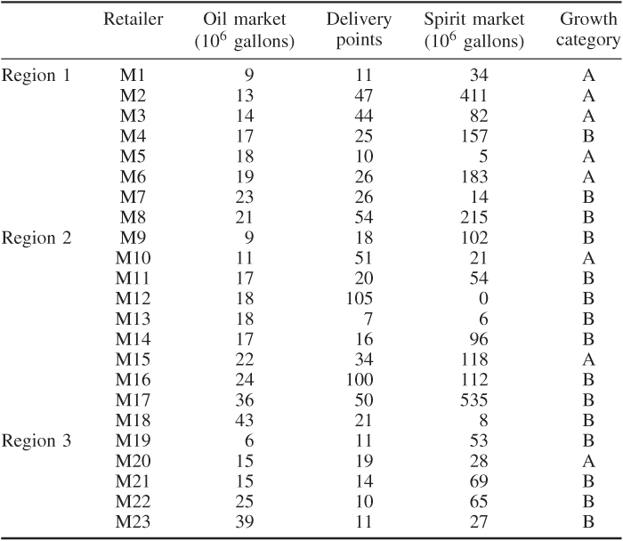
12.13 Market sharing
A large company has two divisions, D1 and D2. The company supplies retailers with oil and spirit. This is a much smaller version of the problem British Petroleum and Shell faced when they were forced to demerge—one of the largest demergers in history. The original model proved impossible to solve in 1972.
It is desired to allocate each retailer to either division D1 or division D2. This division will be the retailer's supplier. As far as possible, this division must be made so that D1 controls 40% of the market and D2 the remaining 60%. The retailers are listed below as M1 to M23. Each retailer has an estimated market for oil and spirit. Retailers M1 to M8 are in region 1; retailers M9 to M18 are in region 2 and retailers M19 to M23 are in region 3. Certain retailers are considered to have good growth prospects and categorised as group A and the others are in group B. Each retailer has a certain number of delivery points as given below. It is desired to make the 40/60 split between D1 and D2 in each of the following respects:
There is a certain flexibility in that any share may vary by ±5%. That is, the share can vary between the limits 35/65 and 45/55.
The primary aim is to find a feasible solution. If, however, there is some choice then possible objectives are (i) to minimise the sum of the percentage deviations from the 40/60 split and (ii) to minimise the maximum such deviation.
Build a model to see if the problem has a feasible solution and if so find the optimal solutions.
The numerical data are given in Table 12.5.
12.14 Opencast mining
A company has obtained permission to opencast mine within a square plot 200 ft × 200 ft. The angle of slip of the soil is such that it is not possible for the sides of the excavation to be steeper than 45°. The company has obtained estimates for the value of the ore in various places at various depths. Bearing in mind the restrictions imposed by the angle of slip, the company decides to consider the problem as one of the extracting of rectangular blocks. Each block has horizontal dimensions 50 ft × 50 ft and a vertical dimension of 25 ft. If the blocks are chosen to lie above one another, as illustrated in vertical section in Figure 12.4, then it is only possible to excavate blocks forming an upturned pyramid. (In a three-dimensional representation, Figure 12.4 would show four blocks lying above each lower block.)
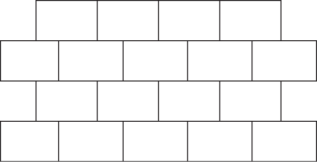
If the estimates of ore value are applied to give values (in percentage of pure metal) for each block in the maximum pyramid, which can be extracted, then the following values are obtained:
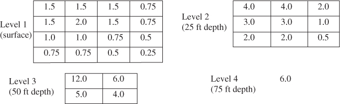
The cost of extraction increases with depth. At successive levels, the cost of extracting a block is as follows:
| Level 1 | £3000 |
| Level 2 | £6000 |
| Level 3 | £8000 |
| Level 4 | £10 000 |
The revenue obtained from a ‘100% value block’ would be £200 000. For each block here, the revenue is proportional to ore value.
Build a model to help decide the best blocks to extract. The objective is to maximise revenue–cost.
The larger version of this problem arose with open-cast iron mining in South Africa.
12.15 Tariff rates (power generation)
A number of power stations are committed to meeting the following electricity load demands over a day:
| 12 p.m. to 6 a.m. | 15 000 MW |
| 6 a.m. to 9 a.m. | 30 000 MW |
| 9 a.m. to 3 p.m. | 25 000 MW |
| 3 p.m. to 6 p.m. | 40 000 MW |
| 6 p.m. to 12 p.m. | 27 000 MW |
There are three types of generating unit available: 12 of type 1, 10 of type 2 and five of type 3. Each generator has to work between a minimum and a maximum level. There is an hourly cost of running each generator at minimum level. In addition, there is an extra hourly cost for each megawatt at which a unit is operated above the minimum level. Starting up a generator also involves a cost. All this information is given in Table 12.6 (with costs in £).
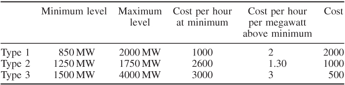
In addition to meeting the estimated load demands there must be sufficient generators working at any time to make it possible to meet an increase in load of up to 15%. This increase would have to be accomplished by adjusting the output of generators already operating within their permitted limits.
Which generators should be working in which periods of the day to minimise total cost?
What is the marginal cost of production of electricity in each period of the day; that is, what tariffs should be charged?
What would be the saving of lowering the 15% reserve output guarantee; that is, what does this security of supply guarantee cost?
12.16 Hydro power
This is an extension of the Tariff Rates (Power Generation) problem of Section 12.15. In addition to the thermal generators, a reservoir powers two hydro generators: one of type A and one of type B. When a hydro generator is running, it operates at a fixed level and the depth of the reservoir decreases. The costs associated with each hydro generator are a fixed start-up cost and a running cost per hour. The characteristics of each type of generator are shown in Table 12.7.
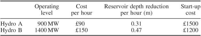
For environmental reasons, the reservoir must be maintained at a depth of between 15 and 20 m. Also, at midnight each night, the reservoir must be 16 m deep. Thermal generators can be used to pump water into the reservoir. To increase the level of the reservoir by 1 m, it requires 3000 MWh of electricity. You may assume that rainfall does not affect the reservoir level.
At any time, it must be possible to meet an increase in demand for electricity of up to 15%. This can be achieved by any combination of the following: switching on a hydro generator (even if this would cause the reservoir depth to fall below 15 m); using the output of a thermal generator, which is used for pumping water into the reservoir; and increasing the operating level of a thermal generator to its maximum. Thermal generators cannot be switched on instantaneously to meet increased demand (although hydro generators can be).
Which generators should be working in which periods of the day, and how should the reservoir be maintained to minimise the total cost?
12.17 Three-dimensional noughts and crosses
Twenty-seven cells are arranged 3 × 3 × 3 in a three-dimensional array as shown in Figure 12.5.
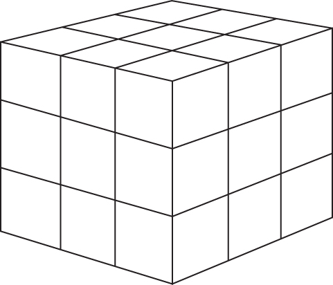
Three cells are regarded as lying in the same line if they are on the same horizontal or vertical line or the same diagonal. Diagonals exist on each horizontal and vertical section and connecting opposite vertices of the cube. (There are 49 lines altogether.)
Given 13 white balls (noughts) and 14 black balls (crosses), arrange them, one to a cell, so as to minimise the number of lines with balls all of one colour.
12.18 Optimising a constraint
In an integer programming problem, the following constraint occurs:
![]()
All the variables occurring in this constraint are 0–1 variables, that is, they can only take the value of 0 or 1.
Find the ‘simplest’ version of this constraint. The objective is to find another constraint involving these variables that is logically equivalent to the original constraint but that has the smallest possible absolute value of the right-hand side (with all coefficients of similar signs to the original coefficients).
If the objective were to find an equivalent constraint where the sum of the absolute values of the coefficients (apart from the right-hand side coefficient) were a minimum what would be the result?
12.19 Distribution 1
A company has two factories, one at Liverpool and one at Brighton. In addition, it has four depots with storage facilities at Newcastle, Birmingham, London and Exeter. The company sells its product to six customers C1, C2, …, C6. Customers can be supplied from either a depot or the factory directly (see Figure 12.6; Table 12.8).
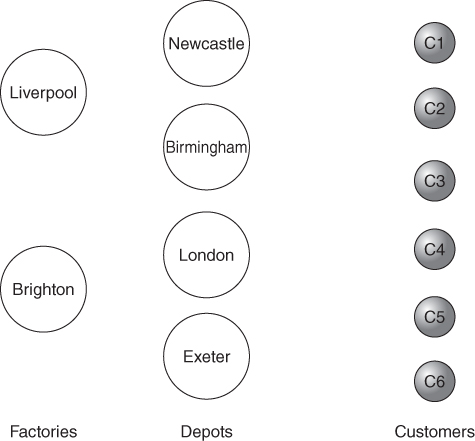
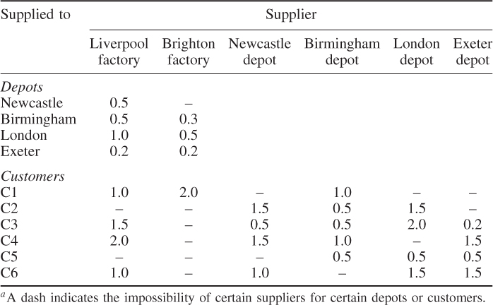
The distribution costs (which are borne by the company) are known; they are given in Table 12.8 (in £ per ton delivered).
Certain customers have expressed preferences for being supplied from factories or depots, which they are used to. The preferred suppliers are as follows:
| C1 | Liverpool (factory) |
| C2 | Newcastle (depot) |
| C3 | No preferences |
| C4 | No preferences |
| C5 | Birmingham (depot) |
| C6 | Exeter or London (depots) |
Each factory has a monthly capacity given as follows, which cannot be exceeded:
| Liverpool | 150 000 tons |
| Brighton | 200 000 tons |
Each depot has a maximum monthly throughput given as follows, which cannot be exceeded:
| Newcastle | 70 000 tons |
| Birmingham | 50 000 tons |
| London | 100 000 tons |
| Exeter | 40 000 tons |
Each customer has a monthly requirement given as follows, which must be met:
| C1 | 50 000 tons |
| C2 | 10 000 tons |
| C3 | 40 000 tons |
| C4 | 35 000 tons |
| CS | 60 000 tons |
| C6 | 20 000 tons |
The company would like to determine the following:
12.20 Depot location (distribution 2)
In the distribution problem, there is a possibility of opening new depots at Bristol and Northampton, as well as of enlarging the Birmingham depot.
It is not considered desirable to have more than four depots and if necessary Newcastle or Exeter (or both) can be closed down.
The monthly costs (in interest charges) of the possible new depots and expansion at Birmingham are given in Table 12.9 together with the potential monthly throughputs.
| Cost (£1000) | Throughput (1000 tons) | |
| Bristol | 12 | 30 |
| Northampton | 4 | 25 |
| Birmingham (expansion) | 3 | 20 |
The monthly savings of closing down the Newcastle and Exeter depots are given in Table 12.10.
| Saving (£1000) | |
| Newcastle | 10 |
| Exeter | 5 |
The distribution costs involving the new depots are given in Table 12.11 (in £ per ton delivered).
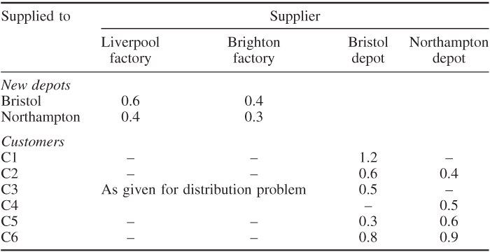
Which new depots should be built? Should Birmingham be expanded? Should Exeter or Newcastle be closed down? What would be the best resultant distribution pattern to minimise overall costs?
12.21 Agricultural pricing
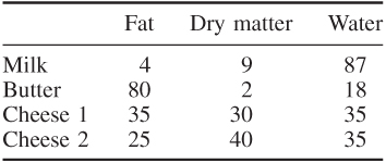
The government of a country wants to decide what prices should be charged for its dairy products, milk, butter and cheese. All these products arise directly or indirectly from the country's raw milk production. This raw milk is usefully divided into the two components as fat and dry matter. After subtracting the quantities of fat and dry matter, which are used for making products for export or consumption on the farms, there is a total yearly availability of 600 000 tons of fat and 750 000 tons of dry matter. This is all available for producing milk, butter and two kinds of cheese for domestic consumption.
The percentage compositions of the products are given in Table 12.12.
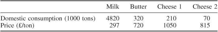
For the previous year, the domestic consumption and prices for the products are given in Table 12.13.
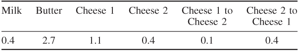
Price elasticities of demand, relating consumer demand to the prices of each product, have been calculated on the basis of past statistics. The price elasticity E of a product is defined by
![]()
For the two makes of cheese, there will be some degree of substitution in consumer demand depending on relative prices. This is measured by cross-elasticity of demand with respect to price. The cross-elasticity EAB from a product A to a product B is defined by
![]()
The elasticities and cross-elasticities are given in Table 12.14.
The objective is to determine what prices and resultant demand will maximise the total revenue.
It is, however, politically unacceptable to allow a certain price index to rise. As a result of the way this index is calculated, this limitation simply demands that the new prices must be such that the total cost of last year's consumption would not be increased. A particularly important additional requirement is to quantify the economic cost of this political limitation.
12.22 Efficiency analysis
A car manufacturer wants to evaluate the efficiencies of different garages, who have received a franchise to sell its cars. The method to be used is data envelopment analysis (DEA). References to this technique are given in Section 3.2. Each garage has a certain number of measurable ‘inputs’. These are taken to be Staff, Showroom Space, Catchment Population in different economic categories and annual Enquiries for different brands of car. Each garage also has a certain number of measurable ‘outputs’. These are taken to be Number Sold of different brands of car and annual Profit. Table 12.15 gives the inputs and outputs for each of the 28 franchised garages.
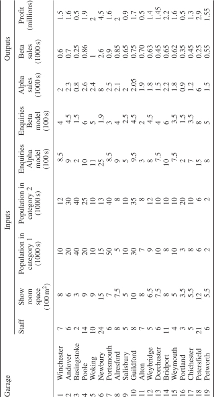
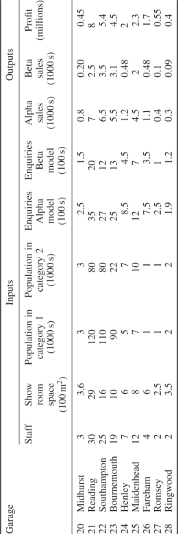
A central assumption of DEA (although modified models can be built to alter this assumption) is that constant returns to scale are possible, that is, doubling a garage's inputs should lead to a doubling of all its outputs. A garage is deemed to be efficient if it is not possible to find a mixture of proportions of other garages, whose combined inputs do not exceed those of the garage being considered, but whose outputs are equal to, or exceed, those of the garage. Should this not be possible then the garage is deemed to be inefficient and the comparator garages can be identified.
A linear programming model can be built to identify efficient and inefficient garages and their comparators.
12.23 Milk collection
A small milk processing company is committed to collecting milk from 20 farms and taking it back to the depot for processing. The company has one tanker lorry with a capacity for carrying 80 000 litres of milk. Eleven of the farms are small and need a collection only every other day. The other nine farms need a collection every day. The positions of the farms in relation to the depot (numbered 1) are given in Table 12.16 together with their collection requirements.
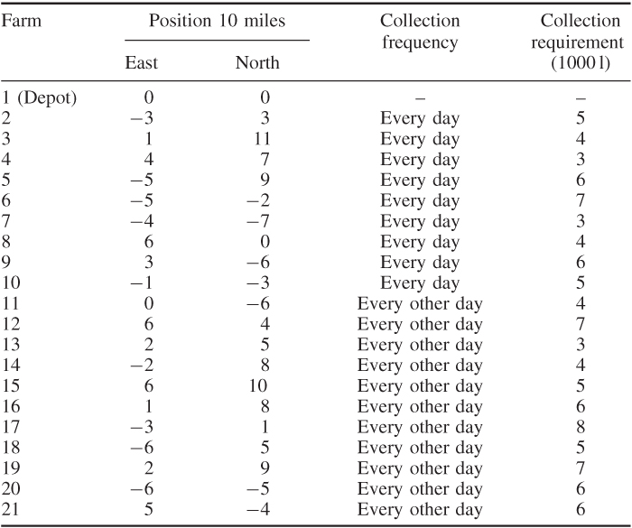
Find the optimal route for the tanker lorry on each day, bearing in mind that it has to (i) visit all the ‘every day’ farms, (ii) visit some of the ‘every other day’ farms and (iii) work within its capacity. On alternate days, it must again visit the ‘every day’ farms and also visit the ‘every other day’ farms not visited on the previous day.
For convenience, a map of the area considered is given in Figure 12.7.

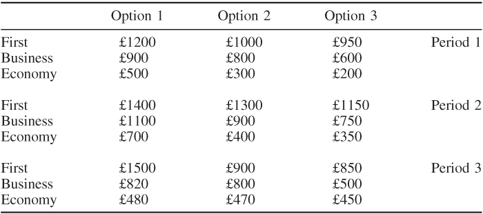
12.24 Yield management
An airline is selling tickets for flights to a particular destination. The flight will depart in three weeks' time. It can use up to six planes each costing £50 000 to hire. Each plane has the following:
Up to 10% of seats in any one category can be transferred to an adjacent category.
It wishes to decide a price for each of these seats. There will be further opportunities to update these prices after one week and two weeks. Once a customer has purchased a ticket, there is no cancellation option.
For administrative simplicity, three price level options are possible in each class (one of which must be chosen). The same option need not be chosen for each class. These are given in Table 12.17 for the current period (period 1) and two future periods.
Demand is uncertain but will be affected by price. Forecasts have been made of these demands according to a probability distribution that divides the demand levels into three scenarios for each period. The probabilities of the three scenarios in each period are as follows:
| Scenario 1 | 0.1 |
| Scenario 2 | 0.7 |
| Scenario 3 | 0.2 |
The forecast demands are shown in Table 12.18.
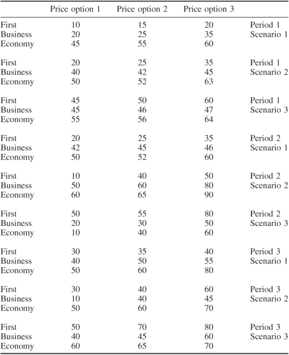
Decide price levels for the current period, how many seats to sell in each class (depending on demand), the provisional number of planes to book and provisional price levels and seats to sell in future periods in order to maximise expected yield. You should schedule to be able to meet commitments under all possible combinations of scenarios.
With hindsight (i.e. not known until the beginning of the next period), it turned out that demand in each period (depending on the price level you chose) was as shown in Table 12.19.
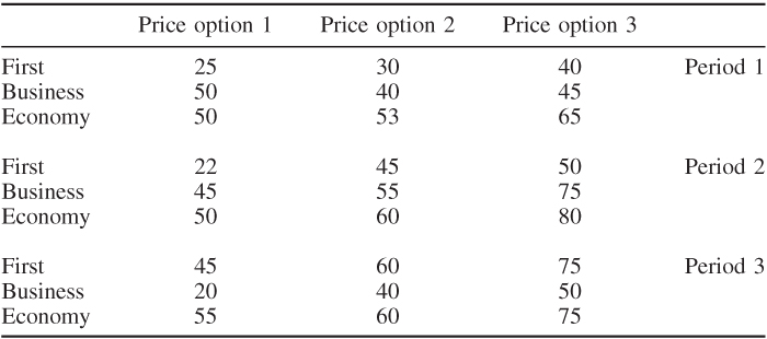
Use the actual demands that resulted from the prices you set in period 1 to rerun the model at the beginning of period 2 to set price levels for period 2 and provisional price levels for period 3.
Repeat this procedure with a rerun at the beginning of period 3. Give the final operational solution.
Contrast this solution to one obtained at the beginning of period 1 by pricing to maximise yield based on expected demands.
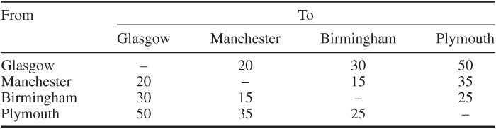
12.25 Car rental 1
A small (‘cut price’) car rental company, renting one type of car, has depots in Glasgow, Manchester, Birmingham and Plymouth. There is an estimated demand for each day of the week except Sunday when the company is closed. These estimates are given in Table 12.20. It is not necessary to meet all demand.
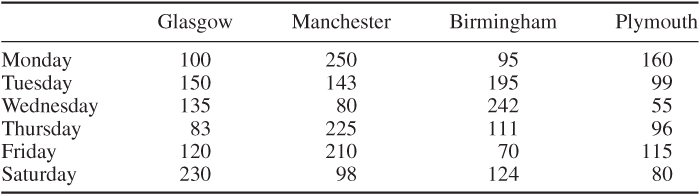
Cars can be rented for one, two or three days and returned to either the depot from which rented or another depot at the start of the next morning. For example, a 2-day rental on Thursday means that the car has to be returned on Saturday morning; a 3-day rental on Friday means that the car has to be returned on Tuesday morning. A 1-day rental on Saturday means that the car has to be returned on Monday morning and a 2-day rental on Tuesday morning.
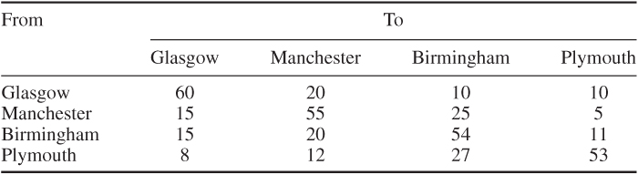
The rental period is independent of the origin and destination. From past data, the company knows the distribution of rental periods: 55% of cars are hired for one day, 20% for two days and 25% for three days. The current estimates of percentages of cars hired from each depot and returned to a given depot (independent of day) are given in Table 12.21.
The marginal cost, to the company, of renting out a car (‘wear and tear’, administration etc.) is estimated as follows:
| 1-Day hire | £20 |
| 2-Day hire | £25 |
| 3-Day hire | £30 |
The ‘opportunity cost’ (interest on capital, storage, servicing, etc.) of owning a car is £15 per week.
It is possible to transfer undamaged cars from one depot to another depot, irrespective of distance. Cars cannot be rented out during the day in which they are transferred. The costs (£), per car, of transfer are given in Table 12.22.
Ten percent of cars returned by customers are damaged. When this happens, the customer is charged an excess of £100 (irrespective of the amount of damage that the company completely covers by its insurance). In addition, the car has to be transferred to a repair depot, where it will be repaired the following day. The cost of transferring a damaged car is the same as transferring an undamaged one (except when the repair depot is the current depot, when it is zero). Again the transfer of a damaged car takes a day, unless it is already at a repair depot. Having arrived at a repair depot, all types of repair (or replacement) take a day.
Only two of the depots have repair capacity. These are (cars/day) as follows:
| Manchester | 12 |
| Birmingham | 20 |
Having been repaired, the car is available for rental at the depot the next day or may be transferred to another depot (taking a day). Thus, a car that is returned damaged on a Wednesday morning is transferred to a repair depot (if not the current depot) during Wednesday, repaired on Thursday and is available for hire at the repair depot on Friday morning.
The rental price depends on the number of days for which the car is hired and whether it is returned to the same depot or not. The prices are given in Table 12.23 (in £).
| Return to Same Depot | Return to Another Depot | |
| 1-Day hire | 50 | 70 |
| 2-Day hire | 70 | 100 |
| 3-Day hire | 120 | 150 |
There is a discount of £20 for hiring on a Saturday so long as the car is returned on Monday morning. This is regarded as a 1-day hire.
For simplicity, we assume the following at the beginning of each day:
In order to maximise weekly profit, the company wants a ‘steady state’ solution in which the same expected number will be located at the same depot on the same day of subsequent weeks.
How many cars should the company own and where should they be located at the start of each day?
This is a case where the integrality of the cars is not worth modelling. Rounded fractional solutions are acceptable
12.26 Car rental 2
In the light of the solution to the problem stated in Section 12.25, the company wants to consider where it might be most worthwhile to expand repair capacity. The weekly fixed costs, given below, include interest payments on the necessary loans for expansion.
The options are as follows:
If any of these options is chosen, it must be carried out in its entirety, that is, there can be no partial expansion. Also, a further expansion at a depot can be carried out only if the first expansion is also carried out, so for example option (2) at Birmingham cannot be chosen unless option (1) is also chosen. If option (2) is chosen, thereby also choosing option (1), these count as two options. Similar stipulations apply regarding the expansions at Manchester. At most three of the options can be carried out.
12.27 Lost baggage distribution
A small company with six vans has a contract with a number of airlines to pick up lost or delayed baggage, belonging to customers in the London area, from Heathrow airport at 6 p.m. each evening. The contract stipulates that each customer must have their baggage delivered by 8 p.m. The company requires a model, which they can solve quickly each evening, to advise them what is the minimum number of vans they need to use and to which customers each van should deliver and in what order. There is no practical capacity limitation on each van. All baggage that needs to be delivered in a two-hour period can be accommodated in a van. Having ascertained the minimum number of vans needed, a solution is then sought, which minimises the maximum time taken by any van.
On a particular evening, the places where deliveries need to be made and the times to travel between them (in minutes) are given in Table 12.24. No allowance is made for drop off times. For convenience, Heathrow will be regarded as the first location.
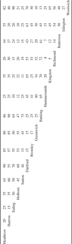
Formulate optimisation models that will minimise the number of vans that need to be used, and within this minimum, minimise the time taken for the longest time delivery.
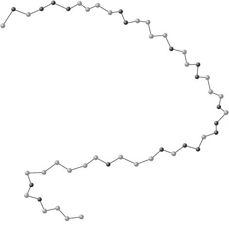
12.28 Protein folding
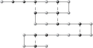
This problem is based on one in the paper by Forrester and Greenberg (2008). It is a simplification of a problem in molecular biology. We take a protein as consisting of a chain of amino acids. For the purpose of this problem, the amino acids come in two forms: hydrophilic (waterloving) and hydrophobic (water hating). An example of such a chain is given in Figure 12.8. with the hydrophobic acids marked in bold.
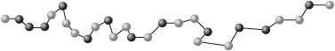
Such a chain naturally folds so as to bring as many hydrophobic acids, as possible, close together. An optimum folding for the chain, in two dimensions, is given in Figure 12.9, with the new matches marked by dashed lines. The problem is to predict the optimum folding. (Forrester and Greenberg also impose a condition that the resultant protein be confined to a given lattice of points. We do not impose that condition here). This problem can be modelled by a number of integer programming formulations. Some of these are discussed in the above reference. Another formulation is suggested in section 13.28. The problem posed here is to find the optimum folding for a chain of 50 amino acids with hydrophobic acids at positions 2, 4, 5, 6, 11, 12, 17, 20, 21, 25, 27, 28, 30, 31, 33, 37, 44 and 46 as shown in Figure 12.10.
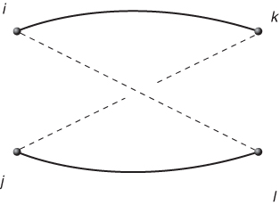
12.29 Protein comparison
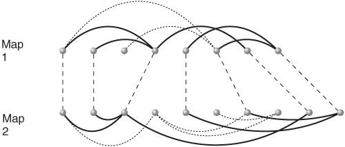
This problem is also based on one in the paper by Forrester and Greenberg (2008). It is concerned with measuring the similarities of two proteins. A protein can be represented by an (undirected) graph with the acids represented by the nodes and the edges being present when two acids are within a threshold distance of each other. This graphical representation is known as the contact map of the protein. Given two contact maps, representing proteins, we would like to find the largest (measured by number of corresponding edges) isomorphic subgraphs in each graph. The acids in each of the proteins are ordered. We need to preserve this ordering in each of the subgraphs, which implies that there can be no crossovers in the comparison. This is illustrated in Figure 12.11. If i < k in the contact map for the first protein then we cannot have l < j in the second protein, if i is to be associated with j and k with l in the comparison.
This problem is well known for being very difficult to solve for even modestly sized proteins.
In Figure 12.12, we give an optimal comparison between two small contact maps leading to 5 corresponding edges.
The problem, we present here, is to compare the contact maps given in Figures 12.13 and 12.14.

