Chapter 2

Solving mathematical programming models

2.1 Algorithms and packages

A set of mathematical rules for solving a particular class of problem or model is known as an algorithm. We are interested in algorithms for solving linear programming (LP), separable programming and integer programming IP models. An algorithm can be programmed into a set of computer routines for solving the corresponding type of model assuming the model is presented to the computer in a specified format. For algorithms that are used frequently, it turns out to be worth writing very sophisticated and efficient computer programmes for use with many different models. Such programmes usually consist of a number of algorithms collected together as a ‘package’ of computer routines. Many such package programmes are available commercially for solving mathematical programming models. They usually contain algorithms for solving LP models, separable programming models and IP models. These packages are written by computer manufacturers, consultancy firms and software houses. They are frequently very sophisticated and represent many person-years of programming effort. When a mathematical programming model is built, it is usually worth making use of an existing package to solve it rather than getting diverted onto the task of programming the computer to solve the model oneself.

The algorithms that are almost invariably used in commercially available packages are (i) the revised simplex algorithm for LP models; (ii) the separable extension of the revised simplex algorithm for separable programming models; and (iii) the branch and bound algorithm for IP models.

It is beyond the scope of this book to describe these algorithms in detail. Algorithms (i) and (ii) are well described in Beale (1968). Algorithm (iii) is outlined in Section 8.3 and well described in Nemhauser and Wolsey (1988). Although the above three algorithms are not the only methods of solving the corresponding models, they have proved to be the most efficient general methods. It should also be emphasized that the algorithms are not totally independent. Hence, the desirability of incorporating them in the same package. Algorithm (ii) is simply a modification of (i) and would use the same computer programme that would make the necessary changes in execution on recognizing a separable model. Algorithm (iii) uses (i) as its first phase and then performs a tree search procedure as described in Section 8.3.

One of the advantages of package programmes is that they are generally very flexible to use. They contain many procedures and options that may be used or ignored as the user thinks fit. We outline some of the extra facilities which most packages offer besides the three basic algorithms mentioned above.

2.1.1 Reduction

Some packages have a procedure for detecting and removing redundancies in a model and so reducing its size and hence time to solve. Such procedures usually go under the name REDUCE, PRESOLVE or ANALYSE. This topic is discussed further in Section 3.4.

2.1.2 Starting solutions

Most packages enable a user to specify a starting solution for a model if he/she wishes. If this starting solution is reasonably close to the optimal solution, the time to solve the model can be reduced considerably.

2.1.3 Simple bounding constraints

A particularly simple type of constraint that often occurs in a model is of the form

where U is a constant. For example, if x represented a quantity of a product to be made, U might represent a marketing limitation. Instead of expressing such a constraint as a conventional constraint row in a model, it is more efficient simply to regard the variable x as having an upper bound of U. The revised simplex algorithm has been modified to cope with such a bound algorithmically (the bounded variable version of the revised simplex). Lower bound constraints such as

need not be specified as conventional constraint rows either but may be dealt with analogously. Most computer packages can deal with bounds on variables in this way.

2.1.4 Ranged constraints

It is sometimes necessary to place upper and lower bounds on the level of some activity represented by a linear expression. This could be done by two constraints such as

A more compact and convenient way to do this is to specify only the first constraint above together with a range of b₁–b₂ on the constraint. The effect of a range is to limit the slack variable (which will be introduced into the constraint by the package) to have an upper bound of b₁–b₂, so implying the second of the above constraints. Most commercial packages have the facility for defining such ranges (not to be confused with ranging in sensitivity analysis, discussed below) on constraints.

2.1.5 Generalized upper bounding constraints

Constraints representing a bound on a sum of variables such as

are very common in many LP models. Such a constraint is sometimes referred to by saying that there is a generalized upper bound (GUB) of M on the set of variables (x₁, x₂, …, x_n). If a considerable proportion of the constraints in a model are of this form and each such set of variables is exclusive of variables in any other set, then it is efficient to use the so-called GUB extension of the revised simplex algorithm. When this is used, it is not necessary to specify these constraints as rows of the model but treat them in a slightly analogous way to simple bounds on single variables. The use of this extension to the algorithm usually makes the solution of a model far quicker.

2.1.6 Sensitivity analysis

When the optimal solution of a model is obtained, there is often interest in investigating the effects of changes in the objective and right-hand side coefficients (and sometimes other coefficients) on this solution. Ranging is the name of a method of finding limits (ranges) within which one of these coefficients can be changed to have a predicted effect on the solution. Such information is very valuable in performing a sensitivity analysis on a model. This topic is discussed at length in Section 6.3 for LP models. Almost all commercial packages have a range facility.

2.2 Practical considerations

In order to demonstrate how a model is presented to a computer package and the form in which the solution is presented, we will consider the second example given in Section 1.2. This blending problem is obviously much smaller than most realistic models but serves to show the form in which a model might be presented.

This problem was converted into a model involving five constraints and six variables. It is convenient to name the variables VEG 1, VEG 2, OIL 1, OIL 2, OIL 3 and PROD. The objective is conveniently named PROF (profit) and the constraints VVEG (vegetable refining), NVEG (non-vegetable refining), UHAR (upper hardness), LHAR (lower hardness) and CONT (continuity). The data are conveniently drawn up in the matrix presented in Table 2.1. It will be seen that the right-hand side coefficients are regarded as a column and named CAP (capacity). Blank cells indicate a zero coefficient.

Table 2.1

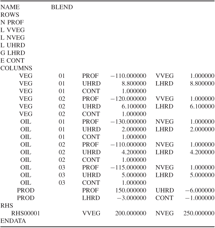
The information in Table 2.1 would generally be presented to the computer through a modelling language. There is, however, a standard format for presenting such information to most computer packages, and almost all modelling languages could convert a model to this format. This is known as MPS (mathematical programming system) format. Other format designs exist, but MPS format is the most universal. The presented data would be as in Table 2.1.

These data are divided into three main sections: the ROWS section, the COLUMNS section and the RHS section. After naming the problem BLEND, the ROWS section consists of a listing of the rows in the model together with a designator N, L, G or E. N stands for a non-constraint row—clearly the objective row must not be a constraint; L stands for a less-than-or-equal (≤) constraint; G stands for a greater-than-or-equal (≥) constraint; E stands for an equality (=) constraint. The COLUMNS section contains the body of the matrix coefficients. These are scanned column by column with up to two non-zero coefficients in a statement (zero coefficients are ignored). Each statement contains the column name, row names and corresponding matrix coefficients. Finally, the RHS section is regarded as a column using the same format as the COLUMNS section. The ENDATA entry indicates the end of the data.

Clearly, it may sometimes be necessary to put in other data as well (such as bounds). The format for such data can always be found from the appropriate manual for a package.

With large models, the solution procedures used will probably be more complicated than the standard ‘default’ methods of the package being used. There are many refinements to the basic algorithms which the user can exploit if he or she thinks it desirable. It should be emphasized that there are few hard-and-fast rules concerning when these modifications should be used. A mathematical programming package should not be regarded as a ‘black box’ to be used in the same way with every model on all computers. Experience with solving the same model again and again on a particular computer with small modifications to the data should enable the user to understand what algorithmic refinements prove efficient or inefficient with the model and computer installation. Experimentation with different strategies and even different packages is always desirable if a model is to be used frequently.

One computational consideration that is very important with large models is mentioned briefly. This concerns starting the solution procedure at an intermediate stage. There are two main reasons why one might wish to do this. First, one might be resolving a model with slightly modified data. Clearly, it would be desirable to exploit one's knowledge of a previous optimal solution to save computation in obtaining the new optimal solution. With linear and separable programming models, it is usually fairly easy to do this with a package, although it is much more difficult for IP models. Most packages have the facility to SAVE a solution on a file. Through the control programme, it is usually possible to RESTORE (or REINSTATE) such a solution as the starting point for a new run. A second reason for wishing to SAVE and RESTORE solutions is that one may wish to terminate a run prematurely. Possibly, the run may be taking a long time and a more urgent job has to go on the computer. Alternatively, the calculations may be running into numerical difficulty and have to be abandoned. In order not to waste the (sometimes considerable) computer time already expended, the intermediate (non-optimal) solution obtained just before termination can be saved and used as a starting point for a subsequent run. It is common to save intermediate solutions at regular intervals in the course of a run. In this way, the last such solution before termination is always available.

2.3 Decision support and expert systems

Some mathematical programming algorithms are incorporated in computer software designed for specific applications. Such systems are sometimes referred to as decision support systems. Often, they are incorporated into management information systems. They usually perform a large number of other functions as well as, possibly, solving a model. These functions probably include accessing databases and interacting with managers or decision makers in a ‘user friendly’ manner. If such systems do incorporate mathematical programming algorithms then many of the modelling and algorithmic aspects are removed from the user who can concentrate on their specific application. In designing and writing such systems, however, it is obviously necessary to automate many of the model building and interpreting procedures discussed in this book.

As decision support systems become more sophisticated, they are likely to present users with possible choices of decision besides the simpler tasks of storing, structuring and presenting data. Such choices may well necessitate the use of mathematical programming, although this function will be hidden from the user.

Another related concept in computer applications software is that of expert systems. These systems also pay great attention to the user interface. They are, for example, sometimes designed to accept ‘informal problem definitions’ and by interacting with users, to help them build up a more precise definition of the problem, possibly in the form of a model. This information is combined with ‘expert’ information built up in the past in order to help decision making. The computational procedures used often involve mathematical programming concepts (e.g. tree searches in IP as described in Section 8.3). While expert systems are beyond the scope of this book, the design and writing of such systems should again depend on mathematical programming and modelling concepts.

The use of mathematical programming in artificial intelligence and expert systems, in particular, is described by Jeroslow (1985) and Williams (1987).

2.4 Constraint programming (CP)

This is a different approach to solving many problems that can also be solved by IP. It is also, sometimes, known as constraint satisfaction or finite domain programming. While the methods used can be regarded as less sophisticated, in a conventional mathematical sense, they use more sophisticated computer science techniques. They have representational advantages that can make problems easier to model and, sometimes, easier to solve in view of the more concise representation. Therefore, we discuss the subject here. It seems likely that hybrid systems will eventually emerge in which the modelling capabilities of constraint programming (CP) are used in modelling languages for systems that use either CP or IP for solving the models. The integration of the two approaches is discussed by Hooker (2011) who has helped to design such a system SIMPL (Yunes et al. (2010)).

In CP, each variable has a finite domain of possible values. Constraints connect (or restrict) the possible combinations of values that the variables can take. These constraints are of a richer variety than the linear constraints of IP (although these are also included) and are usually expressed in the form of predicates, which must be true or false. They are also known as global (or meta) constraints since they are applied (if used) to the model as a whole and incorporated in the CP system used. That is in contrast to ‘local’ or ‘procedural’ constraints which can be constructed by the user to aid the solution process. Conventional IP models use only declarative constraints, so making a clear distinction between the statement of the model and the solution procedure. For illustration, we give some of the more common global constraints that are used in CP systems (often with different names).

all_different (x₁, x₂, …, x_n) means that all the variables in the predicate must take distinct values. While this condition can be modelled by a conventional IP formulation, it is more cumbersome. Once one of the variables has been set to one of the values in its domain (either temporarily or permanently), this predicate implies that the value must be taken out of the domain of the other variables (a process known as constraint propagation). In this way, constraint propagation is used progressively to restrict the domain of the variables until a feasible set of values can be found for each variable, or it can be shown that none exists. This has similarities to REDUCE, PRESOLVE and ANALYSE discussed in Section 3.4 when applied to bound reduction. CP, however, allows ‘domain reduction’ as well as ‘bound reduction’.

Other useful predicates for modelling are

The ≠ predicate stipulated by a constraint of the form a_jx_j ≠ b.

The cardinality predicate written in a form such as card_m (x₁, x₂, …, x_n|v) meaning that exactly m of the variables x₁, x₂, …, x_n must take the value v.

The cumulative ((t₁, t₂, …, t_n), (D₁, D₂, …, D_n), (C₁, C₂, …, C_n), C) predicate restricts n jobs to start at times t₁, t₂, …, t_n when they have durations D₁, D₂, …, D_n consume a resource in amounts C₁, C₂, …, C_n and cannot be using a total of more than C units of the resource at any time.

The circuit (x₁, x₂, …, x_n) predicate stipulates that the numbers x₁, x₂, …, x_n are a permutation of 1, 2, …, n where x_i is the number, in the permutation, occurring after i. Whatsmore, the permutation must be such that it represents a complete circuit, that is, there are no sub-circuits (see Chapter 9 in relation to the travelling salesman problem).

The element (j, (x₁, x₂, …, x_n), z) predicate sets z equal to the jth element in list of variables (x₁, x₂, …, x_n).

The lex − greater predicate can be written in the form (x₁, x₂, …, x_n) > _lex(y₁, y₂, …, y_n). It is true if x₁ = y₁, x₂ = y₂, …, x_r = y_r, x_{r + 1} > y_{r + 1}.

While all the above predicates can be modelled (often in more than one way) using conventional IP variables and constraints, this may be cumbersome and difficult.

There are many more global constraints/predicates available with most commercial CP systems described in the associated manual.

There are a number of situations where CP is more flexible than IP.

For example, it is common, when building an IP model (Chapter 9), to wish to use ‘assignment’ variables such as x_ij = 1 if and only if i is assigned to j. In CP, this would be done by a function f (i) = j.

Another common condition is to wish to specify the ‘inverse’ function, that is, given j, find i such that f (i) = j. This can be done by a version of the element predicate, for example, element (j, f (i), i), which specifies whether the inverse of j is i.

The problems to which CP is applied often exhibit a large degree of symmetry. This may be among the constraints (predicates), solutions or both. For example, i₁, i₂, …, i_n may be identical entities that have to be assigned to entities j₁, j₂, …, j_n. Rather than enumerating all the equivalent solutions, computation can be radically reduced by, for example, using lex − greater to give a priority order to the solutions. This problem also arises with conventional IP models, and improved modelling can also be used there (Chapter 10).

CP is mainly useful where one is trying to find a solution from an often astronomic, number of possibilities. This often happens with combinatorial problems (Chapter 8) where one is trying to find a ‘needle in a haystack’, that is, a solution to a complicated set of conditions where few or none exist. It is less useful where one is seeking an optimal solution to a problem with many feasible solutions, for example, the travelling salesman problem (Chapter 9) or if a problem has no objective function, or all that is sought is a feasible solution. It usually lacks the ability to prove optimality (apart from by imposing successively weaker constraints on the objective until feasibility is obtained). Conventional IP uses the concept of a (usually LP) relaxation (Section 8.3) to restrict the tree search for an optimal solution. This is done since the relaxation gives a bound on the optimal objective value (an upper bound for a maximization or a lower bound for a minimization). This gives it great strength. However, CP uses more sophisticated branching strategies than IP. Such algorithmic considerations are beyond the scope of this book.

There is considerable interest in using predicates, such as those used in CP, for modelling in IP (and then converting to a conventional IP formulation). An early paper by McKinnon and Williams (1989) shows how all the constraints of any IP model can be formulated using the nested at_least_m (x₁, x₂, …, x_n|v) (meaning ‘at least m of x₁, x₂, …, x_n must take the value v’) predicate. Comparisons and connections between IP and CP are discussed by Barth (1995), Bockmayr and Kasper (1998), Brailsford et al. (1996), Proll and Smith (1998), Darby-Dowman and Little (1998), Hooker (1998) and Wilson and Williams (1998). Different ways of formulating the all_different predicate using IP is discussed by Williams and Yan (2001).