Chapter 7

Non-linear models

7.1 Typical applications

It has already been pointed out that many mathematical programming models contain variables representing activities that compete for the use of limited resources. For a linear programming model to be applicable the following must apply:

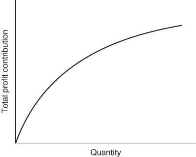
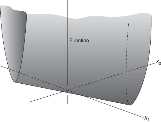
These conditions are clearly applied in the product mix example of Section 1.2 and the result was the linear programming model given there. All the expressions in that model are linear. Nowhere do we get expressions such as , x₁x₂ and log x₁. Suppose, however, that the first of the above conditions did not apply. Instead of each unit of PROD 1 produced contributing £550 to profit, we suppose that the unit profit contribution depends on the quantity of PROD 1 produced. If this unit profit contribution increases with the quantity produced we are said to have increasing returns to scale. For decreases in the unit profit contribution there is said to be decreasing returns to scale. These two situations together with the case of a constant return to scale are illustrated in Figures 7.1-7.3 respectively.

Figure 7.1

Figure 7.2

Figure 7.3

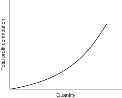
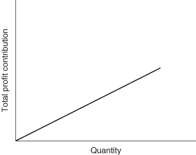
In our product mix model each unit of PROD 1 produced contributes £550 to profit. This gives rise to a term 550x₁, in the objective function. The whole objective function is made up of the sum of similar terms and is said to be linear. As an example of increasing returns to scale we could suppose that the unit profit contribution depended on x₁ and was 550 + 2x₁. This would give rise to the non-linear term in the objective function. We would now have a nonlinear model, although the constraints would still be linear expressions. In practice the non-linear term might not be known explicitly and might simply be represented graphically as shown in Figure 7.1 or 7.2.

As an example of decreasing returns to scale we could suppose that the unit profit contribution was 550/(1 + x₁). This would give rise to the non-linear term 550x₁/(1 + x₁) in the objective function.

The above two cases of non-linearities in the objective function arose through profit margins being affected by increasing or decreasing unit costs arising from increased production. In a similar way unit profit margins will be altered if unit selling price is affected by the volume of production. It frequently happens, in practice, that the unit price, which a product can command, increases with the demand for it. In this case it may be convenient to treat unit selling price as a variable to be determined by the model. For example, if the quantity to be produced is x, the unit cost is c and the unit selling price is p(x), which depends on x, we have

The term p(x)x introduces a non-linearity into the objective function. An obvious first approximation is to take p(x) as a linear function of x. If this is done quadratic terms are introduced into the objective function, resulting in a quadratic programming model. An example of such a model results from the AGRICULTURAL PRICING problem of Part II.

A, sometimes, rather more accurate way to reflect the relationship between p(x) and x is through a price elasticity. We have the following definition of the price elasticity of demand for a good x:

It is possible to regard E_x as constant for the range of values of x and p(x) considered. The above definition then leads to

where k is the price above which the demand is reduced to unity.

For a particular volume of production, x, p(x) gives the unit price at which this level will exactly balance the demand. The resultant non-linear term in the objective function will be

A way in which price elasticities are incorporated in a non-linear programming model of the British National Health Service is described by McDonald et al. (1974).

So far, we have described how mathematical programming models with nonlinear objective functions can arise. Non-linear terms also, sometimes, arise in the constraints of a mathematical programming model.

For example, in a blending problem (such as that described in Example 1.2), a quality (such as hardness) might not depend linearly on the ingredient proportions. Restrictions on such qualities would then give rise to non-linear constraints.

One type of model that has received a certain amount of attention, where non-linearities occur in the constraints, is the geometric programming type of model. Here, the non-linear expressions are all polynomials. For example, we might have the following constraint:

Such models do arise often in engineering problems. They are, however, fairly rare in managerial applications. A full treatment of the subject is given by Duffin et al. (1968).

Non-linear programming models are usually far more difficult to solve than correspondingly sized linear models. It is, however, often possible to solve an approximation to the model through either linear programming or an extension of linear programming known as separable programming. Which case is applicable depends upon an important classification of non-linear models into convex and non-convex problems. This distinction is explained in the next section.

7.2 Local and global optima

Non-linear programming can be divided usefully into convex programming and non-convex programming.

Definition

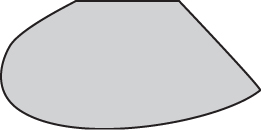
A region of space is said to be convex if the portion of the straight line between any two points in the region also lies in the region.

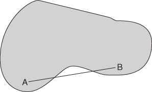
For example, the area shaded in Figure 7.4 is a convex region in two-dimensional space. On the other hand, the area shaded in Figure 7.5 is a non-convex region since A and B are both points within the region yet the line AB between them does not lie entirely in the region.

Figure 7.4

Figure 7.5

Definition

A function f(x) is said to be convex if the set of points (x, y) where y≥ f(x) forms a convex region.

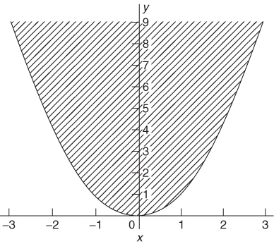
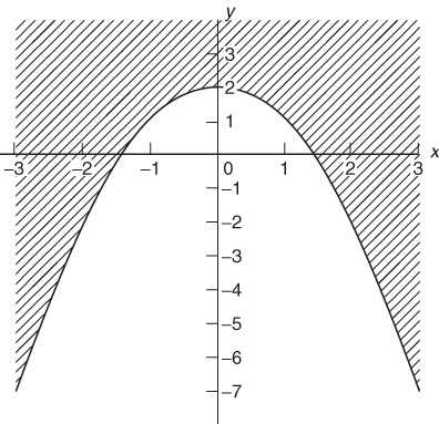
For example, the function x² is convex, as is demonstrated in Figure 7.6 because the shaded area is a convex region. On the other hand, the function 2–x² is non-convex, as is demonstrated in Figure 7.7.

Figure 7.6

Figure 7.7

It should be intuitive that the concepts of convex and non-convex regions and functions apply in as many dimensions as required.

Definition

A mathematical programming model is said to be convex if it involves the minimization of a convex function over a convex feasible region.

Clearly minimizing a convex function is equivalent to maximizing the negation of a convex function. Such a maximization problem will also therefore be convex.

Example 7.1: A Convex Programming Model

The function is represented in Figure 7.8 and easily seen to be convex.

Figure 7.8

This model is represented geometrically in Figure 7.9 with different objective values represented by the curved lines, which arise from contours of the surface in Figure 7.8. Clearly, the optimal solution is represented by point A.

Figure 7.9

It should be obvious that linear programming (LP) is a special case of convex programming. All LP models can be expressed as minimizations, if necessary, of linear functions. A linear function obviously satisfies the definition of a convex function. Moreover, the feasible region defined by a set of linear constraints can easily be shown to be convex.

---

Example 7.2: A Non-convex Programming Model

The function is represented in Figure 7.10 and seen to be non-convex, although, of course, the feasible region of the model in Figure 7.9 is still convex.

Figure 7.10

The model is represented geometrically in Figure 7.11.

Figure 7.11

Again different objective values give rise to the curved lines, which are contours of the surface in Figure 7.10. Clearly, the optimal solution is at C. For a larger problem, however, we would not have the geometrical intuition which we have here. As far as many algorithms (including the separable programming algorithm) are concerned, the point A would also appear as an optimal solution. At A the curved line representing this objective value of −19 deviates away from the feasible region in both directions. This would be taken as evidence in a convex (including linear) programming model that A were the optimal solution. Figure 7.9 demonstrates how the objective contours for a convex problem curve away from the feasible region. For our non-convex example, however, Figure 7.11 demonstrates how the objective contours curve in towards the feasible region and may re-enter it. This, in fact, happens in the example here. The fact that the objective contour passing through A deviates away from the feasible region at A in both directions cannot, therefore, be taken as evidence that it will not re-enter it. In fact, as we can see, it is possible to move out to a better (smaller) objective contour passing through B. Even then we can move out to a still better objective contour passing through C. Points A and B represent what are known as local optima. Many computational procedures (such as separable programming) can guarantee no more than local optima. Clearly, what is really required is a true global optimum such as that represented by point C in Figure 7.11. A fairly graphic way of describing the situation is to consider the problem of a team of mountaineers on a range of mountains in a thick fog. It is easy for them to determine when they are at a local optimum, that is, a mountain peak. The ground will begin to drop in height whichever way they walk. This does not guarantee, however, that there is not another higher mountain peak hidden in the fog. The situation of the mountaineers is similar to that of many non-linear programming algorithms.

---

The possibility of local optima arising from non-convex programming models when certain algorithms are used is what makes such models much more difficult to solve than convex programming models. With a convex programming model any optimum found must be a global optimum. To find a guaranteed global optimum to a non-convex model requires more sophisticated algorithms than the separable programming algorithm described in the next section. A satisfactory, though often computationally expensive, way of tackling such problems is through integer programming as described in Section 9.3.

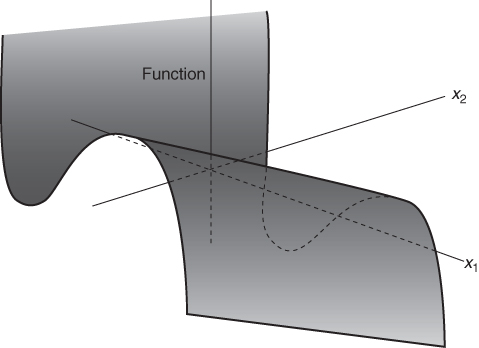
A good illustration of the distinction between convex and non-convex programming models is given by the non-linear programming models mentioned in Section 7.1, which arise when there are diseconomies of scale and economies of scale. The former type of model is convex and the latter non-convex. To see why this is so we first consider the type of cost function that arises when we have diseconomies of scale. This is illustrated in Figure 7.12. If x₁ and x₂ represent quantities of two products to be made, diseconomies of scale will result in the total cost rising faster and faster with increasing values of x₁ and x₂. The result is clearly a convex cost function (to be minimized).

Figure 7.12

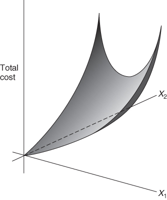
For the case of economies of scale we have the situation represented in Figure 7.13. x₁ and x₂ again represent quantities of two products to be made. As x₁ and x₂ increase, decreasing unit costs result in the total cost rising less and less quickly. The result is clearly a non-convex cost function (to be minimized).

Figure 7.13

7.3 Separable programming

Definition

A separable function is a function that can be expressed as the sum of functions of a single variable.

For example, the function

is separable because each of terms 2x₂ and is a function of a single variable. On the other hand, the function

is not separable because the terms x₁x₂ and x₂/(1 + x₁) are each functions of more than one variable.

The importance of separable functions in a mathematical programming model lies in the fact that they can be approximated to by piecewise linear functions. It is then possible to use separable programming to obtain a global optimum to a convex problem or possibly only a local optimum for a non-convex problem.

Although the class of separable functions might seem to be a rather restrictive one, it is often possible to convert mathematical programming models with non-separable functions into ones with only separable functions. Ways in which this may be done are discussed in Section 7.4. In this way a surprisingly wide class of non-linear programming problems can be converted into separable programming models.

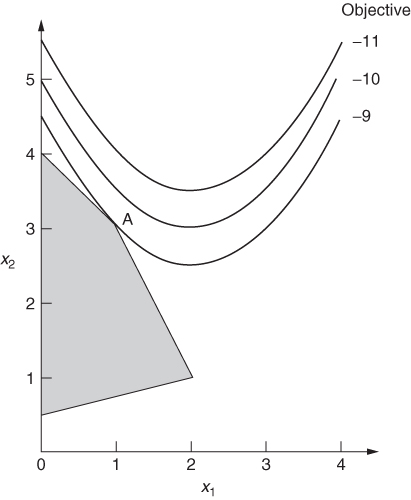
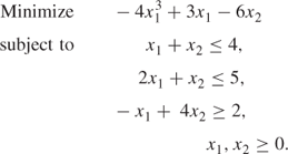
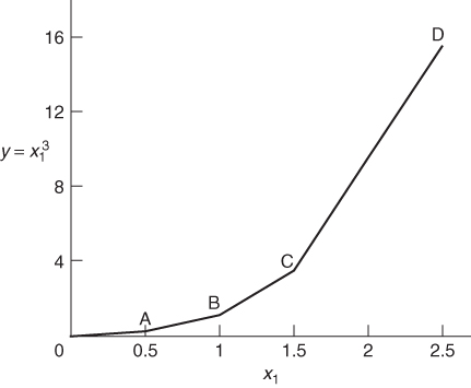
In order to convert a non-linear programming model into a suitable form for separable programming, it is necessary to make piecewise linear approximations to each of the non-linear functions of a single variable. As will become apparent, it does not matter whether the non-linearities are in the objective function or the constraints or both. To illustrate the procedure we will consider the non-linear model given in Example 7.1. The only non-linear term occurring in the model is . A piecewise linear approximation to this function is illustrated in Figure 7.14.

Figure 7.14

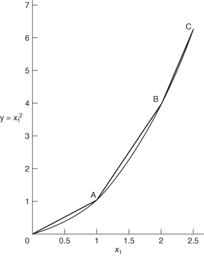
It is easy to see that x₁ can never exceed 2.5 from the second constraint of the problem. The piecewise linear approximation to need, therefore, only be considered for values of x₁ between 0 and 2.5. The curve between 0 and C has been divided into three straight line portions. This inevitably introduces some inaccuracy into the problem. For example, when x₁, is 1.5 the transformed model will regard as 2.5 instead of 2.25. Such inaccuracy can obviously be reduced by a more refined grid involving more straight line portions. For our purpose, however, we will content ourselves with the grid indicated in Figure 7.14. If such an inaccuracy is considered serious, one approach would be to take the value of x, obtained from the optimal solution, refine the grid in the neighbourhood of this value, and re-optimize. Some package programs allow one to do this automatically a number of times, all within one computer run.

Our aim is to eliminate the non-linear term from our model. We can do this by replacing it by the single (linear) term y. It is now possible to relate y to x₁ by the following relationships:

7.1

7.2

7.3

The λ_i are new variables which we introduce into the model. They can be interpreted as ‘weights’ to be attached to the vertices 0, A, B and C. It is, however, necessary to add another stipulation regarding the λ_i:

7.4

The stipulation (7.4) guarantees that corresponding values of x₁ and y lie on one of the straight line segments 0A, AB, or BC. For example if λ₂ = 0.5 and λ₃ = 0.5 (other λ_i being zero) we could get x₁ = 1.5 and y = 2.5. Clearly, ignoring stipulation (7.4) would incorrectly allow the possibility of values x₁ and y off the piecewise straight line 0ABC.

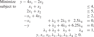
Equations (7.1)–(7.3) give rise to constraints that can be added to our original model (Example 7.1). The term is replaced by y. This results in the following model:

It is important to remember that stipulation (7.4) must apply to the set of variables λ_i. A solution in which, for example, we had and would not be acceptable because this results in the wrong relationship between x₁ and . In general stipulation (7.4) cannot be modelled using linear programming constraints. It can, however, be regarded as a ‘logical condition’ on the variables λ_i and be modelled using integer programming. This is described in Section 9.3. Fortunately, in our example here, no difficulty arises over stipulation (7.4). This is because the original model was convex. Suppose, for example, we were to take as the set of values λ₁ = 0.5, λ₂ = 0.25, λ₃ = 0.25 and λ₄ = 0. This clearly breaks stipulation (7.4). From the relations (7.1) and (7.2) it clearly leads to the point x₁ = 0.75 and y = 1.25 in Figure 7.14. This is above the piecewise straight line. As our objective involves minimizing , we would expect to get a better solution by taking x₁ = 0.75 and y = 0.75 when we drop on to the piecewise straight line. In view of the (convex) shape of the graph we cannot obtain values for the λ_i, which give us points below the piecewise straight line. Therefore, we must always obtain corresponding values of x₁ and y, which lie on one of the line segments by virtue of optimality. Stipulation (7.4) is therefore guaranteed in this case. We can therefore solve our transformed model by linear programming and obtain a satisfactory optimal solution. It is not even necessary to resort to the separable extension of the simplex algorithm that is discussed below. This happens, however, only because our problem is convex.

For a non-convex problem stipulation (7.4) would generally not be satisfied automatically. In order to guarantee that it be satisfied, we could resort to the separable programming modification of the simplex algorithm. In order to demonstrate the difficulty that a non-convex problem presents, we will make a piecewise linear approximation to the non-linear term in the non-convex model of Example 7.2. This is demonstrated in Figure 7.15.

Figure 7.15

This gives us the relationships

As before, the λ_i variables can be interpreted as ‘weights’ attached to the vertices in Figure 7.15.

The λ_i variables must again satisfy the stipulation that at most two adjacent λ_i are non-zero. This time this stipulation is not automatically guaranteed by optimality. Suppose, for example, that we were to obtain the set of values λ₂ = 0.4, λ₃ = 0.5 and λ₄ = 0.1. This would give x₁ = 0.85 and y = 1.3375. The point with these coordinates lies above the piecewise line in Figure 7.15. As our objective function, to be minimized, is dominated by the term our optimization will tend to maximize y. This will tend to take us away from the piecewise line rather than down on to it. In this (non-convex) case it is therefore necessary to use an algorithm which does not allow more than two adjacent λ_i to be non-zero.

The separable programming extension of the simplex algorithm due to Miller (1963) never allows more than two adjacent λ_i into the solution; as a result, it restricts corresponding values of x_i and y to the coordinates of points lying on the desired piecewise straight line.

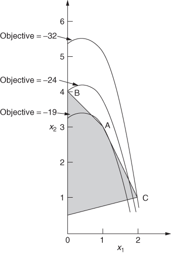
Unfortunately, with non-convex problems, such as Example 7.2, which was modelled above, restricting the values of λ_i to at most two adjacent ones being non-zero does not guarantee any more than a local optimum. We could easily end up at point A or B in Figure 7.11 rather than C.

In both our examples the non-linear functions of a single variable appeared in the objective function. Should such non-linear functions also appear in the constraints the analysis is just the same. They are replaced by linear terms and a piecewise linear approximation made to the non-linear function. Variables λ_i are then introduced in order to relate the new term to the old.

It may not always be easy to decide whether a problem is convex or not. For known convex problems (such as, problems that are linear apart from diseconomies of scale) consisting only of separable functions, piecewise linear approximations are all that are needed. It is not necessary here to use the separable programming algorithm. For problems that are non-convex (such as problems with economies of scale) or where it is not known whether or not they are convex, linear programming is not sufficient. Separable programming can be used but no more than a local optimum can be guaranteed. It is often possible to solve such a model a number of times using different strategies to obtain different local optima. The best of these may then have some chance of being a global optimum. Such computational considerations are, however, beyond the scope of this book, but are sometimes described in manuals associated with particular packages. The only really satisfactory way of being sure of avoiding local optima when a problem is not known to be convex is to resort to integer programming, which is generally much more costly in computer time. This is discussed in Sections 9.2 and 9.3.

Before the end of this section an alternative way of modelling a piecewise linear approximation to a separable function will be described. The formulation method just described is usually known as the λ-form for separable programming where variables λ_i are interpreted as weights attached to the vertices in the piecewise straight line. There is an alternative formulation known as the δ-form. In order to demonstrate the δ-form we reconsider the piecewise linear approximation to the function shown in Figure 7.4. This approximation is redrawn in Figure 7.16.

Figure 7.16

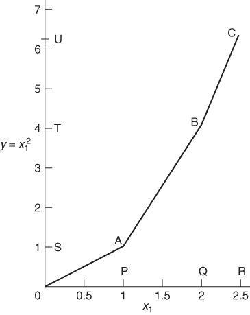
Variables δ₁, δ₂, and δ₃ are introduced to represent proportions of the intervals 0P, PQ, and QR, which are used to make up the value of x₁. We then get

7.5

where

As 0P and PQ are each of length 1, the coefficients of δ₁ and δ₂ in Equation (7.5) are 1. The coefficient of δ₃ is 0.5, reflecting the length of the interval QR.

Similarly,

7.6

where the coefficients of δ₁, δ₂, and δ₃ are now the lengths of the intervals 0S, ST and TU.

In order to ensure that x₁ and y are the coordinates of points on the piecewise lines 0C, we must make the following stipulation:

7.7

Stipulation (7.7) clearly ensures that x₁ and y truly represent distances along their respective axes.

It can be shown that the relaxation associated with the λ-formulation is more constrained than that associated with the δ-formulation. This is the relaxation obtained by dropping the ‘logical’ conditions, (7.4) and (7.7), on the λ and δ variables, as opposed to the LP relaxation obtained by relaxing the IP formulations (see Section 8.3) making it, generally, easier to solve. This was pointed out early on by Williams (1985). When the extra, logical conditions are imposed by integer variables as described in Section 9.3 the λ-formulation can be improved in a way described there.

7.4 Converting a problem to a separable model

The restriction of only allowing non-linear functions to be separable might seem to impose a severe limitation on the class of problems that can be tackled by separable programming. Rather, surprisingly, it is possible to convert a very large class of non-linear programming problems into separable models. When non-separable functions occur in a model, it is often possible to transform the model into one with only separable functions.

A very common non-separable function that occurs in practice is the product of two or more variables. For example, if a term such as x₁x₂ occurs, the model is not immediately a separable one because this is a non-linear function of more than one variable. The model is easily converted into a separable form, however, by the following transformation:

It is easy to see by elementary algebra that is the same as the product x₁x₂ as long as (7.8) and (7.9) are added to the model in the form of equality constraints. The model now contains non-linear functions and of single variables and is therefore separable. These non-linear terms can be dealt with by piecewise linear approximations. It is important to remember that u₂ might need to take negative values. When the possible ranges of values for u₁ and u₂ are considered it may be necessary to either translate u₂ by an appropriate amount or treat it as a ‘free’ variable. A ‘free’ variable in linear programming is one which is not restricted to non-negative values.

Should the product of more than two variables occur in a model (as might happen, for example, in a geometric programming model), then the above procedure could be repeated successively to reduce the model to a separable form.

An alternative way of dealing with product terms in a non-linear model is to use logarithms. We will again consider the example where a product x₁x₂ of two variables occurs in a model, although the method clearly generalizes to larger products. The following transformation can be carried out:

Equation (7.10) gives a non-linear equality constraint to be added to the model. The expression in this constraint is, however, separable as we only have non-linear functions log y, log x₁ and log x₂ of single variables.

Care must be taken, however, when this transformation is made to ensure that neither x₁ nor x₂ (and consequently y) ever take the value 0. If this were to happen their logarithms would become −∞. It may be necessary to translate x₁ and x₂ by certain amounts to avoid this ever happening.

The use of logarithms to convert a non-linear model to a suitable form does, however, sometimes lead to computational problems. Beale (1975) suggests that this can happen if both a variable and its logarithm occur together in the same model. If these are likely to be of widely different orders of magnitude, numerical inaccuracy may lead to computational difficulties.

Non-linear functions of more than one variable (such as product terms) can be dealt with in yet another way by generalizing a piecewise linear approximation to more dimensions. A more complex relationship then has to be specified between the λ_i. As with non-convex separable models, this is only really satisfactorily dealt with through integer programming and is described in Section 9.3.

Many other non-linear functions of more than one variable can be reduced to non-linear functions of a single variable by the addition of extra variables and constraints. Ingenuity is often required but the range of non-linear programming problems that can be made separable in this way is vast. Such transformations do, however, often greatly increase the size of a model and hence the time to solve it.