Chapter 9

Building integer programming models I

9.1 The uses of discrete variables

When integer variables are used in a mathematical programming model, they may serve a number of purposes. These are described below.

9.1.1 Indivisible (discrete) quantities

This is the obvious use mentioned at the beginning of Chapter 8 where we wish to use a variable to represent a quantity that can only come in whole numbers such as aeroplanes, cars, houses or people.

9.1.2 Decision variables

Variables are frequently used in integer programming (IP) to indicate which of a number of possible decisions should be made. Usually, these variables can only take the two values, zero or one. Such variables are known as zero–one (0–1) (or binary) variables. For example, δ = 1 indicates that a depot should be built and δ = 0 indicates that a depot should not be built. We usually adopt the convention of using the Greek letter ‘δ’ for 0 − 1 variables and reserve Latin letters for continuous (real or rational) variables.

It is easy to ensure that a variable, which is also specified to be integer, can only take the two values 0 or 1 by giving the variable a simple upper bound (SUB) of 1. (All variables are assumed to have a simple lower bound of 0 unless it is stated to the contrary).

Although decision variables are usually 0 − 1, they need not always be. For example we might have γ = 0 indicates that no depot should be built; γ = 1 indicates that a depot of type A should be built; γ = 2 indicates that a depot of type B should be built.

9.1.3 Indicator variables

When extra conditions are imposed on a linear programming (LP) model, 0 − 1 variables are usually introduced and ‘linked’ to some of the continuous variables in the problem to indicate certain states. For example, suppose that x represents the quantity of an ingredient to be included in a blend. We may well wish to use an indicator variable δ to distinguish between the state where x = 0 and the state where x > 0. By introducing the following constraint, we can force δ to take the value 1 when x > 0:

9.1

where M is a constant coefficient representing a known upper bound for x.

Logically, we have achieved the condition

9.2

where ‘→’ stands for ‘implies’.

In many applications, Equation (9.2) provides a sufficient link between x and δ (e.g. Example 9.1 below). There are applications (e.g. Example 9.2 below), however, where we also wish to impose the condition

9.3

Equation (9.3) is another way of saying

9.4

Together, Equations (9.2) and (9.3) (or Equation (9.4)) impose the condition

9.5

where ‘↔’ stands for ‘if and only if’.

It is not possible totally to represent Equation (9.3) (or Equation (9.4)) by a constraint. On reflection, this is not surprising. Equation (9.4) gives the condition ‘if δ = 1 , the ingredient represented by x must appear in the blend’. Would we really want to distinguish in practice between no usage of the ingredient and, say, one molecule of the ingredient? It would be much more realistic to define some threshold level m below which we regard the ingredient as unused. Equation (9.4) can now be rewritten as

9.6

This condition can be imposed by the constraint

9.7

 

It should be pointed out that any constant coefficient M can be chosen in constraints of type in Equation (9.1) so long as M is sufficiently big not to restrict the value of x to an extent not desired in the problem being modelled. In practical situations, it is usually possible to specify such a value for M. Although theoretically any sufficiently large value of M will suffice, there is computational advantage in making M as realistic as possible. This point is explained further in Section 10.1 of Chapter 10. Similar considerations apply to the coefficient m in constraints of type in Inequality (9.7).

It is possible to use indicator variables in a similar way to show whether an inequality holds or does not hold. First, suppose that we wish to indicate whether the following inequality holds by means of an indicator variable δ

The following condition is fairly straightforward to formulate. We therefore model it first:

9.11

Equation (9.11) can be represented by the constraint

9.12

where M is an upper bound for the expression ∑ _ja_jx_j − b. It is easy to verify that Inequality (9.12) has the desired effect, that is, when δ = 1 the original constraint is forced to hold and when δ = 0, no constraint is implied.

A convenient way of constructing Inequality (9.12) from condition (9.11) is to pursue the following train of reasoning. If δ = 1 we wish to have ∑ _ia_jx_j–b ≤ 0, that is, if (1–δ) = 0, we wish to have ∑ _ia_jx_j–b ≤ 0. This condition is imposed if

where M is a sufficiently large number. In order to find how large M must be, we consider the case δ = 0, giving ∑ _ja_jx_j–b ≤ M.

This shows that we must choose M sufficiently large that this does not give an undesired constraint. Clearly, M must be chosen to be an upper bound for the expression ∑ _ja_jx_j–b. Rearranging the constraint we have obtained with the variables on the left, we obtain Inequality (9.12).

We now consider how to model the reverse of constraint (9.11), that is,

9.13

This is conveniently expressed as

9.14

that is,

9.15

In dealing with the expression ∑ _ja_jx_j > b, we run into the same difficulties that we met with the expression x > 0. We must rewrite

where is some small tolerance value beyond which we will regard the constraint as having been broken. Should the coefficients a_j be integers as well as the variables x_j, as often happens in this type of situation, there is no difficulty as can be taken as 1.

Equation (9.15) may now be rewritten as

9.16

Using an argument similar to that above, we can represent this condition by the constraint

9.17

where m is a lower bound for the expression

Should we wish to indicate whether a ‘≥’ inequality such as

holds or not by means of an indicator variable δ, the required constraints can easily be obtained by transforming the above constraint into a ‘≤’ form. The corresponding constraints to Inequalities (9.12) and (9.17) above are

9.18

9.19

where m and M are again lower and upper bounds respectively on the expression

Finally, to use an indicator variable δ for an ‘=’ constraint such as

is slightly more complicated. We can use δ = 1 to indicate that the ‘≤’ and ‘≥’ cases hold simultaneously. This is done by stating both the constraints (9.12) and (9.18) together.

If δ = 0, we want to force either the ‘≤’ or the ‘≥’ constraint to be broken. This may be done by expressing Inequalities (9.17), (9.18), (9.19) with two variables δ ′ and δ ″ giving

9.20

9.21

The indicator variable δ forces the required condition by the extra constraint

9.22

In some circumstances, we wish to impose a condition of the type (9.11). Alternatively, we may wish to impose a condition of the type (9.13) or impose both conditions together. These conditions can be dealt with by the linear constraints (9.12) or (9.17) taken individually or together.

In all the constraints derived in this section it is computationally desirable to make m and M as realistic as possible.

9.2 Logical conditions and 0–1 variables

In Section 9.1, it was pointed out that 0–1 variables are often introduced into an LP (or sometimes an IP) model as decision variables or indicator variables. Having introduced such variables, it is then possible to represent logical connections between different decisions or states by linear constraints involving these 0–1 variables. It is at first sight rather surprising that so many different types of logical condition can be imposed in this way.

Some typical examples of logical conditions that can be so modelled are given below. Further examples are given by Williams (1977).

It will be convenient to use some notation from Boolean algebra in this section. This is the so-called set of connectives given below:

These connectives are used to connect propositions denoted by P, Q, R, etc., x > 0, x = 0, δ = 1, etc.

For example, if P stands for the proposition ‘I will miss the bus’ and Q stands for the proposition ‘I will be late’, then P → Q stands for the proposition ‘If I miss the bus, then I will be late’. ∼ P stands for the proposition ‘I will not miss the bus’.

As another example suppose that X_i stands for the proposition ‘Ingredient i is in the blend’ (i ranges over the ingredients A, B and C). Then X_A → (X_B ∨ X_C) stands for the proposition ‘If ingredient A is in the blend then ingredient B or C (or both) must also be in the blend’. This expression could also be written as (X_A → X_B) ∨ (X_A → X_C).

It is possible to define all these connectives in terms of a subset of them. For example, they can all be defined in terms of the set {∨,∼} Such a subset is known as a complete set of connectives. We do not choose to do this and will retain the flexibility of using all the connectives listed above. It is important, however, to realize that certain expressions are equivalent to expressions involving other connectives. We give all the equivalences below that are sufficient for our purpose.

To avoid unnecessary brackets, we consider the symbols ‘∼’, ‘⋅’, ‘∨’ and ‘→’ as each being more binding than their successor when written in this order.

For example,

9.27

9.28

9.29

9.30

9.31

9.32

9.33

9.34

Expressions (9.33) and (9.34) are sometimes known as De Morgan's laws.

Although Boolean algebra provides a convenient means of expressing and manipulating logical relationships, our purpose here is to express these relationships in terms of the familiar equations and inequalities of mathematical programming. (In one sense, we are performing the opposite process to that used in the pseudo-Boolean approach to 0–1 programming mentioned in Section 8.3.)

We will suppose that indicator variables have already been introduced in the manner described in Section 9.1 to represent the decisions or states that we want logically to relate.

It is important to distinguish propositions and variables at this stage. We use X_i to stand for the proposition δ_i = 1 where δ_i is a 0–1 indicator variable. The following propositions and constraints can easily be seen to be equivalent:

9.35

9.36

9.37

9.38

9.39

To illustrate the conversion of a logical condition into a constraint we consider an example.

It is sometimes suggested that polynomial expressions in 0–1 variables are useful for expressing logical conditions. Such polynomial expressions can always be replaced by linear expressions with linear constraints, possibly with a considerable increase in the number of 0–1 variables. For example, the constraint

9.50

represents the condition

9.51

More generally, if a product term such as δ₁δ₂ were to appear anywhere in a model, the model could be made linear by the following steps:

9.53

An example of the need to linearize products of 0–1 variables in this way arises in the DECENTRALIZATION problem in Part III. Products involving more than two variables can be progressively reduced to single variables in a similar manner.

A major defect of the above formulation is that, if there are n original 0–1 variables, there can be up to n(n − 1) new 0–1 variables and 3n(n − 1) extra constraints. A much more compact formulation is due to Glover (1975). Suppose we consider all the terms involving δ₁ in an expression and group them together, for example, δ₁(2δ₂ + 3δ₃ − δ₄). We represent this expression by a new continuous variable w. Then the relations between w and the δ_i are as follows:

We model this by

It should be noted, however, that if there relatively few ‘connections’ between the variables, that is, each variable forms few products with more than one other variable, there may be little saving in the size of model.

It is even possible to linearize terms involving a product of a 0–1 variable with a continuous variable. For example the term xδ, where x is continuous and δ is 0–1, can be treated in the following way:

Other non-linear expressions (such as ratios of polynomials) involving 0–1 variables can also be made linear in similar ways. Such expressions tend to occur fairly rarely and are not therefore considered further. They do, however, provide interesting problems of logical formulation using the principles described in this section and can provide useful exercises for the reader.

The purpose of this section together with Example 9.4 has been to demonstrate a method of imposing logical conditions on a model. This is by no means the only way of approaching this kind of modelling. Different rule-of-thumb methods exist for imposing the desired conditions. Experienced modellers may feel that they could derive the constraints described here by easier methods. It has been the author's experience, however, that the following are true:

A system for automating the formulation of logical conditions within standard predicates and implementing them within the language PROLOG is described by McKinnon and Williams (1989).

Logical conditions are sometimes expressed within a constraint logic programming language as discussed in Section 2.4. The ‘tightest’ way (this concept is explained in Section 8.3) of expressing certain examples using linear programming constraints is described by Hooker and Yan (1999) and Williams and Yan (2001). There is a close relationship between logic and 0–1 integer programming, which is explained in Williams (1995, 2009), Williams and Brailsford (1999) and Chandru and Hooker (1999).

9.3 Special ordered sets of variables

Two very common types of restriction arise in mathematical programming problems for which the concept special ordered set of type 1 (SOS1) and special ordered set of type 2 (SOS2) have been developed. This concept is due to Beale and Tomlin (1969).

An SOS1 is a set of variables (continuous or integer) within which exactly one variable must be non-zero.

An SOS2 is a set of variables within which at most two can be non-zero. The two variables must be adjacent in the ordering given to the set.

It is perfectly possible to model the restrictions that a set of variables belongs to an SOS1 set or an SOS2 set using integer variables and constraints. The way in which this can be done is described below. There is great computational advantage to be gained, however, from treating these restrictions algorithmically. The way in which the branch and bound algorithm can be modified to deal with SOS1 and SOS2 sets is beyond the scope of this book. It is described in Beale and Tomlin.

Some examples are given on how SOS1 sets and SOS2 sets can arise.

 

Although the most common application of SOS1 sets is to modelling what would otherwise be 0–1 integer variables with a constraint such as in Equation (9.59), there are other applications.

The most common application of SOS2 sets is to modelling non-linear functions as described by the following example.

The formulation of a non-linear function in Example 9.7 demands that the non-linear function be separable, that is, the sum of non-linear functions of a single variable. It was demonstrated in Section 7.4 how models with non-separable functions may sometimes be converted into models where the non-linearities are all functions of a single variable. While this is often possible, it can be cumbersome, increasing the size of the model considerably as well as the computational difficulty. An alternative is to extend the concept of an SOS set to that of a chain of linked SOS sets. This has been done by Beale (1980). The idea is best illustrated by a further example.

Some of the problems presented in Part II can be formulated to take advantage of special ordered sets. In particular, DECENTRALIZATION and LOGIC DESIGN can exploit SOS1.

While it is desirable to treat SOS sets algorithmically if this facility exists in the package being used, the restrictions that they imply can be imposed using 0–1 variables and linear constraints. This is now demonstrated.

Suppose (x₁, x₂, …, x_n) is an SOS1 set. If the variables are not 0–1, we introduce 0–1 indicator variables δ₁, δ₂, …, δ_n and link them to the x_i variables in the conventional way by constraints:

9.68

9.69

where M_i and m_i are constant coefficients being upper and lower bounds respectively for x_i.

The following constraint is then imposed on the δ_i variables:

9.70

If the x_i variables are 0–1, we can immediately regard them as the δ_i variables above and only need impose the constraint (9.70).

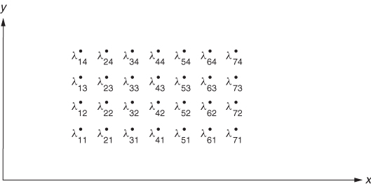
To model an SOS2 set using 0–1 variables is more complicated. Suppose (λ₁, λ₂, …, λ_n) is an SOS2 set. We introduce 0–1 variables together with the following constraints:

9.71

and

9.72

This formulation suggests the relationship between SOS1 and SOS2 sets as Equation (9.72) could be dispensed with by regarding the δ_i as belonging to an SOS1 set as long as the δ_i each have an upper bound of 1.

An improvement to the IP modelling of the λ-formulation has been proposed by Sherali (2001). The formulation gives a tighter LP relaxation and also allows the modelling of discontinuous piecewise linear expressions such as that illustrated in Figure 9.3. In order to define the function uniquely at the point of discontinuity, we must make it upper or lower semi-continuous at the point of discontinuity, that is, define the left or right-hand interval to be open at this point.

In order to model a piecewise linear function, we associate two (weighting) variables λL, λR, which must sum to 1, with each end of each section. Then we stipulate that exactly one pair of weights is positive, confining the function to exactly one of the sections. The IP formulation of the function illustrated in Figure 9.3 is

9.73

9.74

9.75

9.76

9.4 Extra conditions applied to linear programming models

As the majority of practical applications of IP give rise to mixed integer programming models where extra conditions have been applied to an otherwise LP model, this subject is considered further in this section. A number of the commonest applications are briefly outlined.

9.4.1 Disjunctive constraints

Suppose that for an LP problem we do not require all the constraints to hold simultaneously. We do, however, require at least one subset of constraints to hold. This could be stated as

9.77

where R_i is the proposition ‘The constraints in subset i are satisfied’ and constraints 1, 2, …, N form the subset in question. Expression (9.77) is known as a disjunction of constraints.

Following the principles of Section 9.1, we introduce N indicator variables δ_i to indicate whether the R_i are satisfied. In this case, it is only necessary to impose the conditions

9.78

This may be done by constraints of type (9.12) or (9.18) (Section 9.1) taken singly or together according to whether R_i are ‘≤’, ‘≥’, or ‘=’ constraints. We can then impose condition (9.77) by the constraint

9.79

An alternative formulation of Expression (9.77) is possible. This is discussed in Section 10.2 and is due to Jeroslow and Lowe (1984), who report promising computational results in Jeroslow and Lowe (1985).

A generalization of Expression (9.77) that can arise is the condition

9.80

This is modelled in a similar way but using the constraint below in place of Inequality (9.79):

9.81

A variation of expression (9.80) is the condition

9.82

To model Expression (9.82) using indicator variables δ_i, it is only necessary to impose the conditions

9.83

This may be done by constraints of type (9.17) or (9.19) (Section 9.1) taken together or singly according to whether R_i is a ‘≤’, ‘≥’, or ‘=’ constraint. Condition (9.82) can then be imposed by the constraint

9.84

Disjunctions of constraints involve the logical connective ‘∨’ (‘or’) and necessitate IP models.

It is worth pointing out that the connective ‘⋅’ (‘and’) can obviously be coped with through conventional LP as a conjunction of constraints simply involves a series of constraints holding simultaneously. In this sense, one can regard ‘and’ as corresponding to LP and ‘or’ as corresponding to IP.

9.4.2 Non-convex regions

As an application of disjunctive constraints, we show how restrictions corresponding to a non-convex region may be imposed using IP. It is well known that the feasible region of an LP model is convex. (Convexity is defined in Section 7.2.) There are circumstances, however, in non-linear programming problems where we wish to have a non-convex feasible region. For example, we consider the feasible region ABCDEFGO of Figure 9.4. This is a non-convex region bounded by a series of straight lines. Such a region may have arisen through the problem considered or represent a piecewise linear approximation to a non-convex region bounded by curves.

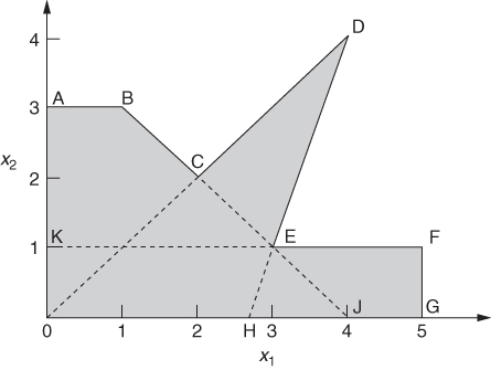
We may conveniently think of the region ABCDEFGO as made up of the union of the three convex regions ABJO, ODH and KFGO, as shown in Figure 9.4. The fact these regions overlap does not matter.

Region ABJO is defined by the constraints

9.85

Region ODH is defined by the constraints

9.86

Region KFGO is defined by the constraints

9.87

We introduce indicator variables δ₁, δ₂ and δ₃ to use in the following conditions:

9.88

9.89

9.90

Equations (9.88), (9.89), (9.90) are respectively imposed by the following constraints:

9.91

9.92

9.93

It is now only necessary to impose the condition that at least one of the set of Inequalities (9.85), (9.86) or (9.87) must hold. This is done by the constraint

9.94

It would also be possible to cope with a situation in which the feasible region was disconnected in this way.

There is an alternative formulation for a connected non-convex region, such as that above, so long as the line joining the origin to any feasible point lies entirely within the feasible region. Seven ‘weighting’ variables λ_A, λ_B, …, λ_G are associated with the vertices A, B, …, G and incorporated in the following constraints:

9.95

9.96

9.97

The λ variables are then restricted to form an SOS2. Notice that this is a generalization of the use of an SOS2 set to model a piecewise linear function such as that represented by the line ABCDEFG. In that case, constraint (9.97) would become an equation, that is, the λs would sum to 1. For the example here, we simply relax this restriction to give a ‘≤’ constraint.

9.4.3 Limiting the number of variables in a solution

This is another application of disjunctive constraints. It is well known that, in LP, the optimal solution need never have more variables at a non-zero value than there are constraints in the problem. Sometimes it is required, however, to restrict this number still further (to k). To do this requires IP. Indicator variables δ_i are introduced to link with each of the n continuous variables x_i in the LP problem by the condition

9.98

As before, this condition is imposed by the constraint

9.99

where M_i is an upper bound on x_i.

We then impose the condition that at most k of the variables x_i can be non-zero by the constraint

A very common application of this type of condition is in limiting the number of ingredients in a blend. The FOOD MANUFACTURE 2 example of Part II is an example of this. Another situation in which the condition might arise is where it is desired to limit the range of products produced in a product mix type LP model.

9.4.4 Sequentially dependent decisions

It sometimes happens that we wish to model a situation in which decisions made at a particular time will affect decisions made later. Suppose, for example, that in a multi-period LP model (n periods) we have introduced a decision variable γ_t into each period to show how a decision should be made in each period. We let γ_t represent the following decisions: γ_t = 0 means the depot should be permanently closed down; γ_t = 1 means the depot should be temporarily closed (this period only); γ_t = 2 means the depot should be used in this period. Clearly, we would wish to impose (among others) the conditions

9.100

This may be done by the following constraints:

9.101

In this case, the decision variable γ_t can take three values. More usually, it will be a 0–1 variable.

A case of sequentially dependent decisions arises in the MINING problem of Part II.

9.4.5 Economies of scale

It was pointed out in Chapter 7 that economies of scale lead to a non-linear programming problem where the objective is equivalent to minimizing a non-convex function. In this situation, it is not possible to reduce the problem to an LP problem by piecewise linear approximations alone. Nor is it possible to rely on separable programming as local optima might result.

Suppose, for example, that we have a model where the objective is to minimize cost. The amount to be manufactured of a particular product is represented by a variable x. For increasing x, the unit marginal costs decrease.

Diagrammatically, we have the situation shown in Figure 9.5. This may be the true cost curve or be a piecewise linear approximation.

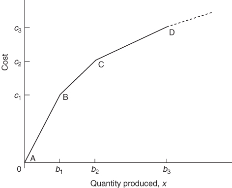
The unit marginal costs are successively

Using the λ-formulation of separable programming as described in Chapter 7, we introduce n + 1 variables λ_i (i = 0, 1, 2, …, n) that may be interpreted as ‘weights’ attached to the vertices A, B, C, D, etc. We then have

9.102

9.103

The set of variables (λ₀, λ₁, …, λ_n) is now regarded as a special ordered set of type 2. If IP is used, a global optimal solution can be obtained.

It is also, of course, possible to model this situation using the δ-formulation of separable programming.

9.4.6 Discrete capacity extensions

It is sometimes unrealistic to regard an LP constraint (usually a capacity constraint) as applying in all circumstances. In real life, it is often possible to violate the constraint at a certain cost. This topic has already been mentioned in Section 3.3. There, however, we allowed this constraint to be relaxed continuously. Often this is not possible. Should the constraint be successively relaxed, it may be possible that it can only be done in finite jumps, for example, we buy in whole new machines or whole new storage tanks.

Suppose the initial right-hand side (RHS) value is b₀ and that this may be successively increased to b₁, b₂, …, b_n.

We have

9.104

also

where 0 < c₁ < c₂ < ··· < c_n.

This situation may be modelled by introducing 0–1 variables. δ₀, δ₁, δ₂, etc., to represent the successive possible RHS values applying. We then have

9.105

The following expression is added to the objective function:

9.106

The set of variables (δ₀, δ₁, …, δ_n) may be treated as an SOS1 set. If this is done, then the δ_i can be regarded as continuous variables having a generalized upper bound of 1, that is, the integrality requirement may be ignored.

9.4.7 Maximax objectives

Suppose we had the following situation:

This is analogous to the minimax objective discussed in Section 3.2 but unlike that case, it cannot be modelled by linear programming.

We can, however, treat it as a case of a disjunctive constraint and use integer programming. The model can be expressed as

9.5 Special kinds of integer programming model

The purpose of this section is to describe some well-known special types of IP model that have received considerable theoretical attention. By describing the structure of these types of model, it is hoped that the model builder may be able to recognize when he or she has such a model. Reference to the extensive literature and computational experience on such models may then be of value.

It should, however, be emphasized that most practical IP models do not fall into any of these categories but arise as MIP models often extending an existing LP model. The considerable attention that has been paid to the IP problems described below should not disguise their limited but nevertheless sometimes significant practical importance.

9.5.1 Set covering problems

These problems derive their name from the following type of abstract problem.

We are given a set of objects that we number as the set S = (1, 2, 3, …, m). We are also given a class of subsets of S. Each of these subsets has a cost associated with it.

The problem is to ‘cover’ all members of S at minimum cost using members of .

For example, suppose S = (1, 2, 3, 4, 5) and = ((1, 2), (1, 3, 5), (2, 4, 5), (3), (1), (4, 5)) and all members of have cost 1.

A cover for S would be (1, 2), (1,3,5) and (2, 4, 5).

In order to obtain the minimum cost cover of S in this example, we could build a 0–1 PIP model. The variables δ_i have the following interpretation:

Constraints are introduced to ensure that each member of S is covered. For example, in order to cover the member 1 of S, we must have at least one of the members (1, 2), (1, 3, 5), or (1) of in the cover. This condition is imposed by constraint (9.107) below. The other constraints ensure a similar condition for the other members of S.

If the objective is simply to minimize the number of members of S used in the cover, the resultant model is as follows:

9.107

9.108

9.109

9.110

9.111

Alternatively, the variables could be given non-unit cost coefficients in the objective.

This model has a number of important properties:

Property 9.1

The problem is a minimization and all constraints are ‘≥’.

Property 9.2

All RHS coefficients are 1.

Property 9.3

All other matrix coefficients are 0 or 1.

As a result of the abstract set covering application described above, all 0–1 PIP models with the above three properties are known as set covering problems.

Generalizations of the problem exist. If property 9.2 is relaxed and we allow larger positive integers than 1 for some RHS coefficients, we obtain the weighted set covering problem. An interpretation of this is that some of the members of S are to be given greater ‘weight’ in the covering than others, that is, they must be covered a certain number of times.

Another generalization that sometimes occurs is when we relax property 9.2 above but also relax property 9.3 to allow matrix coefficients 0 or ±1. This gives rise to the generalized set covering problem.

The best known application of set covering problems is to aircrew scheduling. Here, the members of S can be regarded as ‘legs’ that an airline has to cover and the members of are possible ‘rosters’ (or rotations) involving particular combinations of flights. A common requirement is to cover all legs over some period of time using the minimum number of crews. Each crew is assigned to a roster.

A comprehensive list of applications of set covering problems is given by Balas and Padberg (1975).

Special algorithms do exist for set covering problems. Two such algorithms are described in Chapter 4 of Garfinkel and Nemhauser (1972).

Set covering problems have an important property that often makes them comparatively easy to solve by the branch and bound method. It can be shown that the optimal solution to a set covering problem must be a vertex solution in the same sense as for LP problems. Unfortunately, this vertex solution will not generally be (but sometimes is) the optimal vertex solution to the corresponding LP model. It is, however, often possible to move from this continuous optimum to the integer optimum in comparatively few steps.

The difficulty of solving set covering problems usually arises not from their structure but from their size. In practice, models frequently have comparatively few constraints but an enormous number of variables. There is often considerable virtue in generating columns for the model in the course of optimization. Column generation forms the subject of Section 9.6.

9.5.2 Set packing problems

These problems are closely related to set covering problems. The name again derives from an abstract problem that we first describe.

We are given a set of objects which we number as the set S = (1, 2, 3, …, m). We are also given a class of subsets of S each of which has a certain value associated with it.

The problem is to ‘pack’ as many of the members of into S as possible to maximize total value but without any overlap.

For example, suppose S = (1, 2, 3, 4, 5, 6) and = ((1, 2, 5), (1, 3), (2, 4), (3, 6), (2, 3, 6)). A pack for S would be (1, 2, 5) and (3, 6).

Again we could build a 0 − 1 PIP model to help solve the problem. The variables δ_i have the following interpretation:

Constraints are introduced to ensure that no member of S is included in more than one member of in the pack, that is, there shall be no overlap. For example, in order that the member 2 shall not be included more than once we cannot have more than one of (1, 2, 5), (2, 4) and (2, 3, 6) in the pack. This condition gives rise to the constraint (9.113) below. The other constraints ensure similar conditions for the other members of S.

The objective here is to maximize the number of members of S we can ‘pack in’. For this example the model is

9.112

9.113

9.114

9.115

9.116

9.117

(Constraints (9.115) and (9.116) are obviously redundant.)

Like the set covering problem, this model has a number of important properties:

Property 9.4

The problem is a maximization and all constraints are ‘≤’.

Property 9.5

All RHS coefficients are 1.

Property 9.6

All other matrix coefficients are 0 or 1.

An interesting observation is that the LP problem associated with a set packing problem with objective coefficients of 1 is the dual of the LP problem associated with a set covering problem with objective coefficients of 1. This result is of little obvious significance as far as the optimal solutions to the IP problems are concerned as there may be a ‘duality gap’ between these solutions. This term is explained in Section 10.3. Although a set packing problem with objective coefficients of 1 is the ‘dual’ of a set covering problem with objective coefficients of 1 in this sense, it should be realized that the set S that we wish to cover with members of is not the same as the set S that we wish to pack with members of another class of subsets . The two examples used above to illustrate set covering and set packing problems are so chosen as to be dual problems in this sense, but the set S and class of subsets are different.

As with the set covering problem there are generalizations of the set packing problem obtained by relaxing some of the properties 9.4–9.6 above. If property 9.5 is relaxed and we allow positive integral RHS coefficients greater than 1, we obtain the weighted set packing problem. If we relax property 9.5 as above together with property 9.6 to allow matrix coefficients of 0 or ±1, we obtain the generalized set packing problem.

A special sort of packing problem is known as the matching problem. This problem can be represented by a graph in which the objects S to be packed are nodes. Each subset from S consists of two members of S and is represented by an arc of the graph whose end points represent the two members of S. The problem then becomes one of matching (or pairing) as many vertices as possible together. Extensive work on this problem has been done by Edmonds (1965).

Set packing problems are equivalent to the class of set partitioning problems, which we consider next. Applications and references are described there.

9.5.3 Set partitioning problems

In this case, we are, as before, given a set of objects that we number as the set S = (1,2,3, …, m) and a class of subsets of S.

The problem this time is both to cover all the members of S using members of and also to have no overlap. We, in this sense, have a combined covering and packing problem. There is no useful purpose in distinguishing between maximization and minimization problems here. Both may arise.

As an example, we consider the same S and used in the example to describe the set covering problem. The difference is that we must now impose stricter conditions to ensure that each member of S is in exactly one member of the partition (or cover and pack combined). This is done by making the constraints (9.107)–(9.111)‘=’ instead of ‘≥’, giving

9.118

9.119

9.120

9.121

9.122

For example, a feasible partition of S consists of (1, 2), (3) and (4, 5).

An easily understood way in which the set partitioning problem can arise is again in aircrew scheduling. Suppose that we did not allow aircrews to travel as passengers on other flights. It would then be necessary that each member of S (a leg) be covered by exactly one member of (a roster). We would then have a set partitioning problem in place of the set covering problem.

Another application of the set partitioning problem is to political districting. In this problem, there is usually an extra constraint fixing the total number of political districts (or constituencies). The objective is usually to minimize the maximum deviation of the electorate in a district from the average electorate in a district. This minimax objective can be dealt with in the way described in Section 3.3. A reference to tackling the problem by IP is Garfinkel and Nemhauser (1970).

We now show the essential equivalence between set partitioning and set packing problems. If we introduce slack variables into each of the ‘≤’ constraints of a set packing problem, we obtain ‘=’ constraints. These slack variables can only take the values 0 or 1 and could therefore be regarded with all the other variables in the problems as 0 − 1 variables. The result would clearly be a set partitioning problem.

To show the converse is slightly more complicated. Suppose we have a set partitioning problem. Each constraint will be of the form

9.123

We introduce an extra 0 − 1 variable δ into constraint (9.123) giving

9.124

If the problem is one of minimization, δ can be given a sufficiently high positive cost M in the objective to force δ to be zero in the optimal solution. For a maximization problem, making M a negative number with a sufficiently high absolute value has the same effect. Instead of introducing S explicitly into the objective function, we can substitute the expression below derived from Equation (9.124):

9.125

There is no loss of generality in replacing Equation (9.124) by the constraint

9.126

If similar transformations are performed for all the other constraints, the set partitioning problem can be transformed into a set packing problem.

Hence we obtain the result that set packing problems and set partitioning problems can easily be transformed from one to the other. Both types of problem possess the property mentioned in connection with the set covering problems, that is, the optimal solution is always a vertex solution to the corresponding LP problem.

The set partitioning (or packing) problem is generally even easier to solve than the set covering problem. It is easy to see from the small numerical example that a set partitioning problem by using ‘=’ constraints is more constrained than the corresponding set covering problem. Likewise, the corresponding LP problem is more constrained. It will be seen in Section 10.1 that constraining the corresponding LP problem to an IP problem as much as possible is computationally very desirable.

A comprehensive list of applications and references to the set packing and partitioning problems is given by Balas and Padberg (1975). Chapter 4 of Garfinkel and Nemhauser (1972) treats these problems very fully and gives a special purpose algorithm. Ryan (1992) describes how the set partitioning problem can be applied to aircrew scheduling.

In view of its close similarity to set partitioning and packing problems it is rather surprising that the set covering problem has some important differences. Although the set covering problem is an essentially easy type of problem, to solve it is distinctly more difficult than the former problems. It is possible to transform a set partitioning (or packing) problem into a set covering problem by introducing an extra 0 − 1 variable with a negative coefficient in Equation (9.123) and performing analogous substitutions to those described above. The reverse transformation of a set covering problem to a set partitioning (or packing) problem is not, however, generally possible, revealing the distinctness of the problems.

9.5.4 The knapsack problem

A PIP model with a single constraint is known as a knapsack problem. Such a problem can take the form

9.127

where γ₁, γ₂, …, γ_n ≥ 0 and take integer values.

The name ‘knapsack’ arises from the rather contrived application of a hiker trying to fill her knapsack to maximum total value. Each item she considers taking with her has a certain value and a certain weight. An overall weight limitation gives the single constraint.

An obvious extension of the problem is where there are additional upper bounding constraints on the variables. Most commonly, these upper bounds will all be 1 giving a 0 − 1 knapsack problem.

Practical applications occasionally arise in project selection and capital budgeting allocation problems if there is only one constraint. The problem of stocking a warehouse to maximum value given that the goods stored come in indivisible units also gives rise to an obvious knapsack problem.

The occurrence of such immediately obvious applications is, however, fairly rare. Much more commonly, the knapsack problem arises in LP and IP problems where one generates the columns of the model in the course of optimization. As such techniques are intimately linked with the algorithmic side of mathematical programming, they are beyond the scope of this book. The original application of the knapsack problem in this way was to the cutting stock problem. This is described by Gilmore and Gomory (1963, 1965) (and in Section 9.6).

In practice, knapsack problems are comparatively easy to solve. The branch and bound method is not, however, an efficient method to use. If it is desired to solve a large number of knapsack problems (e.g. when generating columns for an LP or IP model), it is better to use a more efficient method. Dynamic programming proves an efficient method of solving knapsack problems. This method and further references are given in Chapter 6 of Garfinkel and Nemhauser (1972).

9.5.5 The travelling salesman problem

This problem has received a lot of attention largely because of its conceptual simplicity. The simplicity with which the problem can be stated is in marked contrast to the difficulty of solving such problems in practice.

The name ‘travelling salesman’ arises from the following application.

A salesman has to set out from home to visit a number of customers before finally returning home. The problem is to find the order in which he or she should visit all the customers in order to minimize the total distance covered.

Generalizations and special cases of the problem have been considered. For example, sometimes it is not necessary that the salesman return home. Often, the problem itself has special properties, for example, the distance from A to B is the same as the distance from B to A. The vehicle routing problem can be reduced to a travelling salesman problem. This is the problem of organizing deliveries to customers using a number of vehicles of different sizes. The reverse problem of picking up deliveries (e.g. letters from post office boxes) given a number of vehicles (or postal workers) can also be treated in this way. This problem is considered below.

Job sequencing problems in order to minimize set-up costs can be treated as travelling salesman problems where the ‘distance between cities’ represents the ‘set-up cost between operations’. A not very obvious (nor probably practical) application of this sort is to sequencing the colours that are used for a single brush in a series of painting operations. Obviously, the transition between certain colours will require a more thorough cleaning of the brush than a transition between other colours. The problem of sequencing the colours to minimize the total cleaning time gives rise to a travelling salesman problem.

The travelling salesman problem can be formulated as an IP model in a number of ways. We present one such formulation here. Any solution (not necessarily optimal) to the problem is referred to as a ‘tour’.

Suppose the cities to be visited are numbered 0, 1, 2, …, n. 0–1 integer variables δ_ij are introduced with the following interpretation:

The objective is simply to minimize ∑ _{i, j}c_ijδ_ij, where c_ij is the distance (or cost) between i and j.

There are two obvious conditions that must be fulfilled:

9.128

9.129

Condition (9.128) is achieved by the constraints

9.130

Condition (9.129) is achieved by the constraints

9.131

As the model has so far been presented, we have an assignment problem as described in Section 5.3. Unfortunately, the constraints (9.130) and (9.131) are not sufficient. Suppose, for example, we were considering a problem with eight cities (n = 7). The solution drawn in Figure 9.6 would satisfy all the conditions (9.130) and (9.131).

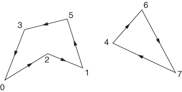
Clearly, we cannot allow subtours such as those shown here.

The problem of adding extra constraints so as to avoid subtours proves quite difficult. In practice, it is often desirable to add these constraints in the course of optimization as subtours arise. For example, as a result of the solution to the ‘relaxed problem’ exhibited by Figure 9.6, we would add the extra constraint

9.132

This would rule out any subtour around the cities 4, 6 and 7 (and implicitly around 0, 1, 2, 3 and 5 if these were the only other cities). Potentially, there are an exponential number of such subtour elimination constraints, and it would be impractical to state them all explicitly. Therefore, they are added on an ‘as needed’ basis as above. In practice, one rarely needs to add more than a very small fraction of this exponential number before a solution without subtours is obtained. When this happens, we clearly have the optimal solution.

There are ingenious ways of producing non-exponential sized formulations by the introduction of new variables or replacing the variables by new ones with a different interpretation.

However, all except one of these formulations have weaker LP relaxations than the conventional formulation, which is due to Dantzig et al. (1954). Orman and Williams (2006) give eight different formulations and show (surprisingly) that one can rank the strengths of their LP relaxations, independently of problem instance. They classify the non-exponential formulations into three distinct forms. A sequential formulation is due to Miller et al. (1960) who introduce extra variables representing the sequence numbers in which cities are visited and use these variables in constraints that prevent subtours. Gavish and Graves (1978) introduce flow variables, which are only allowed in arcs that are used in the tour. These, together with the material balance constraints (Section 5.3) of the network flow problem, prevent subtours. There are a number of variants of this formulation, for example, Finke et al. (1983). In particular, Wong (1980) and Claus (1984) give a multi-commodity network flow formulation, which, remarkably, has the same strength LP relaxation as the conventional formulation. However it has, of the order of n³ variables and constraints, which still makes it impractical to solve the full model in one optimization. Finally time-staged formulations are given by Vajda (1961) and Fox et al. (1980) who use a third index t so as to let the new variables δ_ijt represent whether the salesman goes from city i to city j at stage (‘time’) t .These variables can then be incorporated in constraints to rule out subtours.

A comprehensive survey of the travelling salesman problem is Lawler et al. (1995). There have been dramatic advances in solving the problem fairly recently. Applegate et al. (2006) discuss the computational side. Special algorithms have been developed. One of the most successful is that of Held and Karp (1971).

There are also variants and extensions of the travelling salesman problem. One such is the MILK COLLECTION problem described in Part II. This is based on a paper by Butler et al. (1997). Another is the LOST BAGGAGE DISTRIBUTION problem also described in Part II.

9.5.6 The vehicle routing problem

This is, practically, the most important extension of the travelling salesman problem where one has to schedule a number of vehicles, of limited capacity, around a number of customers. Hence, in addition to the sequencing of the customers to be visited (the travelling salesman problem) one has to decide which vehicles visit which customers. Each customer has a known demand (assumed to be of one commodity, although it is possible, easily to extend to more than one commodity). Hence the limited vehicle capacities have to be taken into account. In addition, there are often time window conditions requiring that certain customers can only receive deliveries between certain times. We give a formulation of this problem as an extension of that of the travelling salesman problem mentioned above. As with that formulation, it is generally necessary to add extra constraints to break subtours in the course of optimization.

Let δ_ijk = 1 iff vehicle k goes directly from customer i to customer j,

γ_ik = 1 iff vehicle k visits customer i, (apart from the depot),

τ_i = time at which customer i is visited.

We assume that each customer (apart from the depot, regarded as customer 0) is visited by exactly one vehicle, that is, there are no ‘split’ deliveries to a customer. For data, we assume there are m vehicles and that vehicle k has capacity Q_k and customer i has requirement q_i. Also we assume that the time taken between customers i and j is d_ij and that customer i must take delivery between times a_i and b_i.

There are a number of possible objectives, for example, minimize the number of vehicles needed, minimize total cost or minimize maximum time taken by a vehicle. For illustration, we consider the second objective and assume that the cost (not necessarly proportional to the time) of going from i to j directly is c_ij.

The model is

Such a formulation could prove very difficult to solve for reasonable-sized problem instances. Another approach is to use column generation, which is discussed in Section 9.6. (see also Desrosiers et al. (1984)). In this approach, feasible routes for a vehicle, that is, obeying the capacity and time window constraints, are generated separately from the main model, which then selects and combines them in a feasible and optimal manner.

Variants of this problem are the MILK COLLECTION and LOST BAGGAGE DISTRIBUTION problems given in Part II.

9.5.7 The quadratic assignment problem

This is a generalization of the assignment problem described in Section 5.3. Whereas that problem could be treated as an LP problem and was therefore comparatively easy to solve, the quadratic assignment problem is a genuine IP problem and often very difficult to solve.

As with the assignment problem, we consider the problem as related to two sets of objects S and T. S and T both have the same number of members, which are be indexed 1 to n. The problem is to assign each member of S to exactly one member of T in order to achieve some objective. There are two sorts of conditions we must fulfil:

9.133

9.134

0 − 1 variables δ_ij can be introduced with the following interpretations:

Conditions (9.133) and (9.134) are imposed by the following two types of constraint:

9.135

9.136

The objective is more complex than with the assignment problem. We have cost coefficients c_ijkl, which have the following interpretations. c_ijkl is the cost incurred by assigning i (a member of S) to j (a member of T) at the same time as assigning k (a member of S) to l (a member of T). This cost will clearly be incurred only if δ_ij = 1 and δ_kl = 1, that is, if the product δ_ijδ_kl = 1. The objective then becomes a quadratic expression in 0 − 1 variables:

9.137

The condition k > i on the indices prevents the cost of each pair of assignments being counted twice. It is very common for the coefficients c_ijkl to be derived from the product of other coefficients t_ik and d_jl so that

9.138

In order to understand this rather complicated model, it is worth considering two applications.

Firstly, we consider S to be a set of n factories and T to be a set of n cities. The problem is to locate one factory in each city and to minimize total communication costs between factories. The communication costs depend on (i) the frequency of communication between each pair of factories and (ii) the distances between the two cities where each pair of factories is located.

Clearly, some factories will have little to do with each other and can be located far apart at little cost. On the other hand, some factories may need to communicate a lot. The cost of communication will depend on the distance apart. In this application, we can interpret the coefficients t_ik and d_jl in Equation (9.138) as follows: t_ik is the frequency of communication between factories i and k (measured in appropriate units); d_jl is the cost per unit of communication between cities j and l (clearly, this will be related to the distance between j and l). Obviously, the cost of communication between the factories i and k, located in cities j and l, will be given by Equation (9.138). The total cost is therefore represented by the objective function (9.137).

Another application concerns the placement of n electronic modules in n predetermined positions on a backplate. S represents the set of modules and T represents the set of positions on the backplate. The modules have to be connected to each other by a series of wires. If the objective is to minimize the total length of wire used, we have a quadratic assignment problem similar to the above model. The coefficients t_ik and d_jl have the following interpretations: t_ik is the number of wires that must connect module i to the module k, and d_jl is the distance between position j and position l on the backplate. Many modifications of the quadratic assignment problem described above exist. Frequently conditions (9.133) and (9.134) are relaxed, to allow more than one member of S (or possibly none) to be assigned to a member of T, where S and T may not have the same number of members. A modified problem of this sort is the DECENTRALIZATION example in Part II.

One way of tackling the quadratic assignment problem is to reduce the problem to a linear 0 − 1 PIP problem. It is necessary to remove the quadratic terms in the objective function. Two ways of transforming products of 0 − 1 variables into linear expressions in an IP model were described in Section 9.2. For fairly small models, the first transformation is possible but for larger models, the result can be an enormous expansion in the number of variables and constraints in the model. The solution of a practical problem of this sort by using a similar type of transformation is described by Beale and Tomlin (1972).

A survey of practical applications, as well as other methods of tackling the problem, is given by Lawler (1974). He also shows how a different formulation of the travelling salesman problem, to that given here, leads to a quadratic assignment problem. It should be pointed out, however, that although a travelling salesman problem is often difficult to solve, a quadratic assignment problem of comparable dimensions is usually even harder.

9.6 Column generation

The generation of columns in the course of optimization has already been referred to in the context of decomposition, in Section 4.3 and the set covering and vehicle routing problems in Section 9.5. All the relevant models there are characterized by a very large (often astronomic) number of variables, only a small proportion of which will feature in the optimal solution. Therefore, it seems more efficient only to append them to the model, in the course of optimization, if it seems likely they will be in the optimal solution. Although the method of generation will depend on the nature of the model and the optimization method used, it is still appropriate to consider this general approach in a book on model building. In principle, but not in practice, all the possible variables could be created at the beginning. Column generation is frequently applied to special types of integer programming models. Hence its inclusion in this chapter.

Possible solutions, or components of solutions, are generated separately from the main (master) model (sometimes by optimizations and sometimes by heuristics) and appended to it in the course of optimization. In the case of decomposition, these components are the solutions of subproblems. In the case of the set covering problem, applied to aircrew scheduling, they might be possible rosters generated as paths through a space–time diagram of an airline schedule. For the vehicle routing problem, they would be routes covered by individual vehicles (respecting capacity constaints and time windows).

We illustrate column generation by means of the cutting stock problem, which was one of the original applications decribed by Gilmore and Gomory (1961 and 1963). This can be applied to cutting ordered widths of wallpaper from standard widths to minimize waste or ordered lengths of pipe from standard lengths in order to minimize the number of standard lengths that need to be cut. The cutting stock problem can also be regarded as a special case of the bin packing problem where it is desired to pack a number of items of different sizes into standard size bins so as to minimize the number of bins used.

Suppose a plumber stocks standard lengths of pipe, all of length 19 m. He has orders for

How should he cut these lengths out of his standard lengths so as to minimize the number of standard lengths used?

We firstly give a bad formulation of this problem, as an integer programme, in order to illustrate the advantage of one based on column generation.

Let x_ij = number of pipes of length i (4, 5 or 6 m) cut from standard pipe j numbering the standard, stocked pipes 1, 2, 3, … etc.

The constraints are

The objective is

A major defect of this model is that there will be many symmetrically equivalent solutions, as the standard pipes are indistinguable. Even if symmetry breaking constraints (Section 10.2) are appended, this model would take a very long time to solve (the reader might like to try solving this tiny example using a computer package). We therefore present a much better model based on column generation.

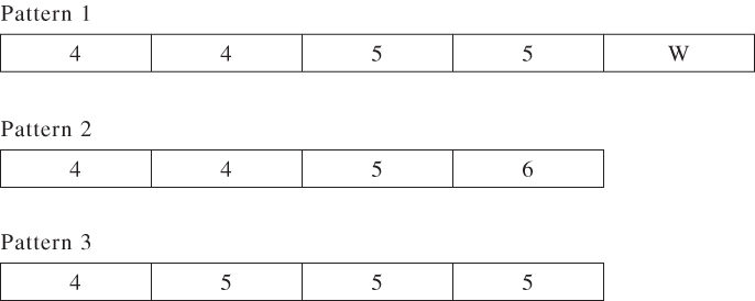
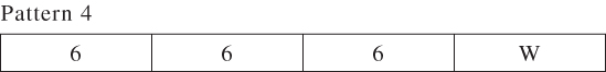
The main constraint above is the second (knapsack) one. The solutions to this constraint are the possible patterns that can be made up out of the standard lengths. We give some of the possible patterns below (including the waste, W) There are obviously more patterns and in a larger example, there will be an astronomic number, most of which will not be used.

A better formulation, using column generation, which finds the minimum number of such patterns needed is

Note that each variable has a column of constraint coefficients corresponding to the number of times each of the order lengths occurs in the pattern. The RHS coefficients are the demands for each length. Solving this model (as an IP) yields γ₁ = 0, γ₂ = 22, γ₃ = 0, requiring 22 standard pipes. Clearly there are better solutions if other patterns are used as well. It is possible to devise other ‘useful’ patterns using the shadow prices from the optimal LP solution to the current model. To start with these shadow prices turn out to be 0, 0, 1. If we were to have a pattern with a lengths of 4 m, b lengths of 5 m and c lengths of 6 m its reduced cost (‘value’ in reducing the objective) would be c − 1. We therefore seek a pattern that maximizes this quantity subject to fitting the pattern into the standard length, that is, we wish to

Clearly a, b, c are integer variables, giving a knapsack problem. This instance has the optimal solution a = b = 0, c = 3, with objective 2, indicating that this pattern will reduce the number of pipes used (in the LP relaxation) giving

Hence we have generated a new column that can be appended to the model to give

This model has optimal IP solution γ₁ = 0, γ₂ = 4, γ₃ = 4, γ₄ = 6. requiring 14 standard pipes. The shadow prices are 1/3, 0, 1/3 which, in order to find another pattern with maximum reduced cost, leads to

This has the optimal solution a = 4, b = 0, c = 0 with objective value 1/3, giving

Appending the column corresponding to this pattern gives

This model gives the same solution as before. In fact, this is the overall optimal solution which has, therefore, been obtained without considering many of the potential patterns.