
Chapter 10
Building integer programming models II
10.1 Good and bad formulations
Most of the considerations of Section 3.4 concerning linear programming (LP) models will also apply to integer programming (IP) models and will not be reconsidered here. There are, however, some important additional considerations that must be taken into account when building IP models. The primary additional consideration is the much greater computational difficulty of solving IP models over LP models. It is fairly common to build an IP model only to find the cost of solving it prohibitive. Frequently, it is possible to reformulate the problem, giving another model that is easier to solve. Such reformulations must often be considered in conjunction with the solution strategy to be employed. It will be assumed throughout that the branch and bound method described in Section 8.3 is to be used.
In some respects, much greater flexibility is possible in building IP models than in building LP models. The flexibility results in a greater divergence between good and bad models of a practical problem. The purpose of this chapter is to suggest ways in which good models may be constructed.
It is convenient to consider variables and constraints separately. There is often the possibility of using many or few variables and many or few constraints in a model. The considerations governing this will be considered.
10.1.1 The number of variables in an IP model
We confine our attention here to the number of integer variables in an IP model as this is often regarded as a good indicator of the computational difficulty.
Suppose we had a 0–1 IP model (either mixed integer or pure integer). If the model had n 0–1 variables, this would indicate 2n possible settings for the variables and hence 2n potential nodes hanging at the bottom of the solution tree. In total there would be 2n + 1 − 1 nodes in such a tree. One might therefore expect the solution time to go up exponentially with the number of 0–1 variables. For quite modest values of n, 2n is very large, for example, 2100 is greater than one million raised to the power 5. The situation is not of course anywhere near as bad as this, as many of the 2n potential nodes will never be examined. The branch and bound method rules out large sections of the potential tree from examination as being infeasible or worse than solutions already known. It is, however, worth pausing to consider the fact that one may sometimes solve 100 0–1 variable IP problems in a few hundred nodes. This represents only about 0.00 … 001 per cent of the potential total where there are 28 zeros after the decimal point. In view of this very surprising efficiency that the branch and bound method exhibits over the potential amount of computation, the number of 0–1 variables is often a very poor indicator of the difficulty of an IP model. We, however, suggest one circumstance in which the number of such variables might be usefully reduced, later in this section. Before doing that, we indicate ways in which the number of integer variables in a model might be increased to good effect.
It is convenient here to describe a well-known device for expanding any general integer variable in a model to a number of 0–1 variables. Suppose γ is a general (non-negative) integer variable with a known upper bound of u (an upper bound is required for all integer variables in an IP model if the branch and bound method is to be used), that is,
![]()
γ may be replaced in this model by the expression
where the δi are 0–1 variables and 2r is the smallest power of 2 greater than or equal to u.
It is easy to see that the expression (10.1) can take any possible integral value between 0 and u by different combinations of values for the δi variables. Clearly, the number of 0–1 variables required in an expansion like this is roughly log2u. In practice, u will probably be fairly small and the number of 0–1 variables produced not too large. If, however, this device were employed on a large number of the variables in the model, the result might be a great expansion in model size. Generally, there will be little virtue in an expansion of this sort except to facilitate the use of some specialized algorithm applying only to 0–1 problems. This is beyond the scope of this book.
Although there is some virtue in keeping an LP model compact, any such advantages that this may imply for the corresponding IP model are usually drowned by other much more important considerations. Using the branch and bound method there is sometimes virtue in introducing extra 0–1 variables as useful variables in the branching process. Such 0–1 variables represent ‘dichotomies’ in the system being modelled. To make such dichotomies explicit can be valuable, as is demonstrated in the following example due to Jeffreys (1974).

10.3 ![]()
10.4 ![]()
10.5 ![]()
In some circumstances, however, there is advantage to be gained in reducing the number of integer variables. One such case is illustrated in the following example. Here the problem exhibits a symmetry, which can be computationally undesirable.
![]()
10.9 ![]()
10.1.2 The number of constraints in an IP model
It was pointed out in Chapter 3 that the difficulty of an LP model is very dependent on the number of constraints. Here we show that in an IP model this effect is often completely drowned by other considerations. In fact, an IP model is often made easier to solve by expanding the number of constraints.
In an LP model, we search for vertex solutions on the boundary of the feasible region. For the corresponding IP model, we are interested in integer points that may well lie in the interior of the feasible region. This is illustrated in Figure 10.1. ABCD is the feasible region of the LP problem but we must confine our attention to the lattice of integer points. For an IP model, the corresponding LP model is known as the LP relaxation.

In this diagram, we assume both x1 and x2 to be integer variables. For mixed integer problems, we are interested in points in an diagram analogous to Figure 10.1, some of whose coordinates are integers, but where other coordinates are allowed to be continuous. Clearly, this situation is difficult to picture in a few dimensions. Suppose, however, that there were a further continuous variable x3 to be considered in Figure 10.1. This would give rise to a coordinate coming out at right angles to the page. Feasible solutions to the mixed integer problem would consist of lines parallel to the x3-axis coming out of the page from the integer points in Figure 10.1. These lines would have, of course, to lie inside the three-dimensional feasible region of the corresponding LP problem.
Ideally, we would like to reformulate the IP model so that the feasible region of the corresponding LP model becomes PQRSTUV. This is known as the convex hull of feasible integer points in ABCD. It is the smallest convex set containing all the feasible integer points. If it were possible to reformulate the IP problem in this way, we could solve the problem as an LP problem as the integrality requirement would automatically be satisfied. Such a formulation, where the LP relaxation gives the convex hull of IP solutions, is known as sharp.
Each vertex (and hence optimal solution) of the new feasible region PQRSTUV is an integer point. Unfortunately, in many practical problems, the effort required to obtain the convex hull of integer points would be enormous and far outweigh the computation needed to solve the original formulation of the IP problem. There are, however, important classes of problems where one of the following can happen:
We consider each of these classes of problems in turn.
Case (i) concerns some problems that have already been considered in Section 5.3. Although superficially these problems might appear to give rise to PIP (pure integer programming) models, the optimal solution of the corresponding LP problem always results in integer values for the integer variables. The model may therefore be treated as an LP problem. Problems falling into this category include the transportation problem, the minimum cost network flow problem and the assignment problem. It is sometimes possible to recognize when an IP model has a structure that guarantees that the corresponding LP model will have an integer optimal solution. Clearly, it is very useful to be able to recognize this property as the high computational cost of IP need not be incurred. Consider the following LP model: Maximize ![]() subject to Ax = b and x ≥ 0.
subject to Ax = b and x ≥ 0.
Here we assume that slack variables have been added to the constraints, if necessary, to make them all equalities. For the above model to yield an optimal solution with all variables integer for every objective coefficient vector c and integer right-hand side b, the matrix A must have a property known as total unimodularity.
Definition
A matrix A is totally unimodular if every square sub-matrix of A has its determinant equal to 0 or ±1.
The fact that this property guarantees that there will be an integer optimal solution to the LP model (for any c and integer b) is proved in Garfinkel and Nemhauser (1972, p. 67). Unfortunately, the above definition of total unimodularity is of little help in detecting the property. To evaluate the determinant of every square sub-matrix would be prohibitive. There is, however, a property (which we call P) that is easier to detect, which guarantees total unimodularity. It is, however, only a sufficient condition, not a necessary condition. Matrices without property P may still be totally unimodular.
Property P
A particular case of the property P is when subset P1 is empty and P2 consists of all the rows of A. Then for the property to hold, we must have all columns consisting of either one non-zero element ±1 or two non-zero elements +1 and −1.
As an example of this property holding, we can consider the small transportation problem of Section 5.3:
10.10 
Each column clearly contains a +1 and a −1, showing the property to hold and hence guaranteeing total unimodularity. There is often virtue in trying to reformulate a model in order to try to capture this easily detected property. The automation of such reformulation (where possible) was described in Section 5.4. In case (ii) below, the dual situation is illustrated.
Although the property above refers to a partitioning of the rows of a matrix A into two subsets, the partitioning could equally well apply to the columns. If A is totally unimodular, its transpose A′ must also be totally unimodular. Again, a particular instance of this property guaranteeing total unimodularity is when each row of the matrix A of an LP model contains a +1 and a −1.
Finally, it should be pointed out that total unimodularity is a strong property that guarantees integer optimal solutions to an LP problem for all c and integer b. Many IP models for which the matrix A is not totally unimodular frequently (although not always) produce integer solutions to the optimal solution of the corresponding LP problem. In particular, this often happens with the set packing, partitioning and covering problems discussed in Section 9.5. There are good reasons why this is likely to happen for these types of problems. Such considerations are, however, fairly technical and beyond the scope of this book. They are discussed in Chapter 8 of Garfinkel and Nemhauser (1972). Properties of A that guarantee integer LP solutions for a specific right-hand side b are discussed by Padberg (1974) for the case of the set partitioning problem.
The discussion of total unimodularity above applies only to PIP models. Clearly, there are corresponding considerations for MIP (mixed integer programming) models, where integer values for the integer variables in the optimal LP solution are guaranteed. Such considerations are, however, very difficult and there is little theoretical work as yet that is of value to practical model builders.
Case (ii) above concerns problems where, with a little thought, a reformulation can result in a model with the total unimodularity property. Consider a generalization of constraint (9.44):
where δi and δ are 0–1 variables.
This kind of constraint arises fairly frequently in IP models and represents the logical condition
10.12 ![]()
Sometimes, this condition is more easily thought of as the logical equivalent condition
10.13 ![]()
It was shown in Section 9.2 that by a different argument, constraint (9.44) of that section can be reformulated using two constraints. A similar reformulation can be applied here, giving the n constraints

Should all the constraints in the model be similar to the constraints of Inequality (10.14) then the dual problem has the property P described above, which guarantees total unimodularity. There is, therefore, great virtue in such a reformulation as the high computational costs associated with an IP problem over an LP problem is avoided. An example of a reformulation of a problem in this way is described by Rhys (1970). He also demonstrates another advantage of the reformulation as yielding a more meaningful economic interpretation of the shadow prices. This topic is considered in Section 10.3. A practical example of a formulation such as that described above is given in Part III where the formulation of the OPENCAST MINING problem is discussed.
Constraint (10.11) above shows the possibility of sometimes reformulating a PIP problem that is not totally unimodular in order to make it totally unimodular. There is also virtue in reformulating an already totally unimodular problem, which we do not know to be totally unimodular, if by so doing we convert it into a form where property P applies. Examples of this are given by Veinott and Wagner (1962) and Daniel (1973). As with case (i), the above discussion of case (ii) only applies to PIP problems. Again, it must be possible (although difficult) to generalize these ideas to MIP problems.
Case (iii) concerns problems where there is either no obvious totally unimodular reformulation or where the problem gives an MIP model. In cases (i) and (ii), we reduced the feasible region to the convex hull of feasible integer points, even though this was not obvious from the algebraic treatment given. It is sometimes possible to go part way towards this aim. Suppose, for example (as might frequently happen in a MIP model), that only some of the constraints were of the form (10.11). By expanding these constraints into the series of constraints (10.14) we would reduce the size of the feasible region of the LP. Even though the existence of other constraints in the problem might result in some integer variables taking fractional values in the LP optimal solution, this solution should be ‘nearer’ the integer optimal solution than would be the case with the original model. The term ‘nearer’ is purposely vague. A reformulation such as this might result in the objective value at node 1 of the solution tree (e.g. Figure 8.1) being closer to the objective value of the optimal integer solution when found. On the other hand, it might result in there being less fractional solution values in the LP optimum. Whatever the result of the reformulation, one would normally expect the solution time for the reformulated model to be less than for the original model. Constraints involving just two coefficients +1 and −1 also arise in models involving sequentially dependent decisions as described in Section 9.4. Such constraints are always to be desired even if their derivation results in an expansion of the constraints of a model. An example of this is the suggested formulation in Part III for the MINING problem.
It is worth indicating in another way why a series of constraints such as in Inequalities (10.14) is preferable to the single constraint (10.11). Although constraints (10.11) and (10.14) are exactly equivalent in an IP sense, they are certainly not equivalent in an LP sense. In fact Inequality (10.11) is the sum of all the constraints in Inequalities (10.14). By adding together constraints in an LP problem, one generally weakens their effect. This is what happens here. Inequality (10.11) admits fractional solutions, which Inequality (10.14) would not admit. For example, the solution
10.15 ![]()
satisfies Inequality (10.11) but breaks Inequalities (10.14) (for n ≥ 3).
Hence, Inequalities (10.14) are more effective at ruling out unwanted fractional solutions.
The ideas discussed above are relevant to the FOOD MANUFACTURE 2 problem, which gives rise to an MIP model and to the DECENTRALIZATION and LOGICAL DESIGN problems, which give rise to PIP models.
Some of the material so far presented in this section was first published by Williams (1974). A discussion of some very similar ideas applied to a more complicated version of the DECENTRALIZATION problem is given in Beale and Tomlin (1972).
It is also relevant here to discuss the value of the coefficient ‘M’ when linking indicator variables to continuous variables by constraints such as in Equations (9.1), (9.12), (9.19) and (9.21). These types of constraints usually (but not always) arise in MIP models.
We will consider the simplest way in which such a constraint arises when we are using a 0–1 variable δ to indicate the condition below on the continuous variable x:
This condition is represented by the constraint
So long as M is a true upper bound for x condition (10.16) is imposed, however large we make M. There is virtue, however, in making M as small as possible without imposing a spurious restriction on x. This is because by making M smaller we reduce the size of the feasible region of the LP problem corresponding to the MIP problem. Suppose, for example, we took M as 1000 when it was known that x would never exceed 100. The following fractional solution would satisfy Inequality (10.17):
10.18 ![]()
but would violate it if M were taken as 100. There are other good reasons for making M as realistic as possible. For example, if M were again taken as 1000, the following fractional solution would satisfy Inequality (10.17):
10.19 ![]()
A small value of δ, such as this, might well fall below the tolerance that indicates whether a variable is integer or not. If it did, δ would be taken as 0, giving the spurious integer solution
10.20 ![]()
If, however, M were made smaller, this would be less likely to happen. Finally, the inadvisability of having coefficients of widely differing magnitudes, as mentioned in Section 3.4, makes a small value of M desirable.
It is also sometimes possible to split up a constraint using a coefficient M in an analogous fashion to the way in which Inequality (10.11) was split up into Inequalities (10.14). This is demonstrated by the following example.
![]()
10.21 ![]()
10.22 
10.23 ![]()
Further ways of reformulating IP models in order to ease their solution are described in the next section.
Before a large IP model is built, it is often a very good idea to build a small version of the model first. Experimentation with different solution strategies, possibly with reformulation, can give one valuable experience before one embarks on the much larger model.
Sometimes, by examining the structure of a model, it is possible to make observations that lead one to a tightening of the constraints. A dramatic example of this (even when the application was unknown) is described by Daniel (1978), resulting in the solution of a reformulated model in 171 nodes where previously the tree search had been abandoned after 4757 nodes.
The automatic reformulation of IP models in order to tighten the LP relaxation is described by Crowder et al. (1983) and Van Roy and Wolsey (1984). The derivation of facet-defining constraints is discussed by Wolsey (1976, 1989).
10.2 Simplifying an integer programming model
In Section 10.1, it was shown that it is often possible to reformulate an IP model in order to create another model that is easier to solve. This is sometimes made possible by considering the practical situation being modelled. In this section, we are concerned with rather less obvious transformations of an IP model. Again, the aim is to make the model easier to solve.
10.2.1 Tightening bounds
In Section 3.4, part of the procedure of Brearley et al. (1975) for simplifying LP models was outlined. The full application of that procedure involves removing redundant simple bounds in an LP model. It is not, however, generally worthwhile removing redundant bounds on an integer variable. Instead it is better to tighten the bounds if possible. The argument for doing this is similar to some of the reformulation arguments used in Section 10.1. By tightening bounds, the corresponding LP problem may be made more constrained resulting in the optimal solution to the LP problem being closer to the optimal IP solution. In order to illustrate the procedure, a small example from Balas (1965) is used. This example was also used in the description of the procedure given by Brearley, Mitra and Williams.
R1 
![]()
![]()
![]()
![]()
![]()
10.2.2 Simplifying a single integer constraint to another single integer constraint
Consider the integer constraint
where γ1 and γ2 are general integer variables. By looking at this constraint geometrically in Figure 10.2, it is easy to see that it may also be written as
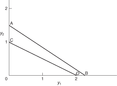
In Figure 10.2, the original constraint (10.23) indicates the feasible points must lie to the left of AB. By shifting the line AB to CD no integer points are excluded from, and no new integer points are included in, the feasible region. CD gives rise to the new constraint (10.24).
Clearly, there are advantages in using constraint (10.24) rather than (10.23) as the feasible region of the corresponding LP problem has been reduced. While constraints such as (10.23) involving general integer variables do not arise very frequently such constraints can occur involving only 0–1 variables. We therefore confine our attention to the 0–1 case. Should more general integer variables be involved, it is, of course, always possible to expand them into 0–1 variables as described in Section 10.1. Our problem is now given a constraint such as
where the δi are 0–1 variables, to re-express it as an equivalent constraint
where Inequality (10.26) is more constrained than Inequality (10.25) in the corresponding LP problem. There is no loss of generality in assuming all the coefficients of Inequalities (10.25) and (10.26) to be non-negative as should a negative coefficient ai occur in Inequality (10.25), the corresponding variable δi may be complemented by the substitution
![]()
making the new coefficient of ![]() positive.
positive.
Clearly ‘≥’ constraints can be converted to ‘≤’. Equality constraints are most conveniently dealt with by converting them into a ‘≤’ together with a ‘≥’ constraint. The result will be two simplified constraints in place of the original single ‘=’ constraint.
The simplification of a pure 0–1 constraint such as in Inequality (10.25) in order to produce the one in Inequality (10.26) can itself be formulated and solved as an LP problem. Rather than present the technical details of the procedure here, a specific problem, OPTIMIZING A CONSTRAINT is given in Part II. The formulation and discussion in Part III should make the general procedure clear.
If the original constraint to be simplified involved general integer variables, rather than 0–1 integer variables, and it is desired to replace it by a constraint in the same variables, then it will be necessary to restrict the new coefficients of the 0–1 form. For example, suppose we had a general integer variable γ (≤7). If its original coefficient were a in the 0–1 form of the constraint, we would have the term
with γ1 + 2γ2 + 4γ3 representing variable γ, where γ1, γ2 and γ3 are 0–1 variables. The resultant simplification would produce an equivalent term
10.28 ![]()
For this term to be replaceable by a term bγ, we would have to ensure that
giving b = b1.
Using the LP formulation described for the 0–1 example in Part II, it would be necessary to impose conditions such as (10.29) as extra LP constraints for the general integer case.
The effort of trying to simplify single integer constraints in this way is often not worthwhile. In many models, these constraints represent logical conditions and are already in their simplest form as single constraints. Applications where such simplification could possibly prove worthwhile are project selection and capital budgeting problems. It also proves worthwhile to simplify single constraints in this way in the MARKET SHARING problem presented in Part II.
The simplification of a single 0–1 constraint into another single 0–1 constraint considered here has been described by Bradley et al. (1974).
10.2.3 Simplifying a single integer constraint to a collection of integer constraints
We again confine our attention to pure 0–1 constraints given that general integer variables can be expanded, if necessary, into 0–1 variables.
It may often be advantageous to express a single 0–1 constraint as a collection of 0–1 constraints. We have already seen this in Section 10.1, where constraint (10.11) was re-expressed as the constraints (10.14). Here, we present a general procedure for expanding any pure 0–1 constraint into a collection of constraints. Ideally, we would like to be able to re-express the constraint by a collection of constraints defining the convex hull of feasible 0–1 solutions. In order to make this clear, we present an example.
10.32 ![]()
10.34 ![]()
10.35 ![]()
10.36 ![]()
Definition
A subset {i1, i2, …, ir} of the indices 1, 2, …, n of the coefficients in Inequality (10.33) will be called a cover if ![]() .
.
Clearly, it is not possible for all the δi corresponding to indices i within a cover to be 1 simultaneously. This condition may be expressed by the constraint
Definition
A cover {i1, i2, …, ir} is said to be a minimal cover if no proper subset of {i1, i2, …, ir} is also a cover.
Definition
A minimal cover {i1, i2, …, ir} can be extended in the following way:
If {i1, i2, …, ir} is a minimal cover, it can be augmented to give an extended cover i1, i2, …, ir + s. The constraint (10.37) corresponding to the minimal cover can correspondingly be extended to
Definition
If a minimal cover gives rise to an extended cover that is not a proper subset of any other extended cover arising from a minimal cover with the same number of indices, the original minimal cover is known as a strong cover.
Balas shows that if an extended cover arises from a strong cover then the constraints such as in Inequality (10.38) encompass all the facets of the convex hull of feasible 0–1 points of Inequality (10.33) that have coefficients 0 or 1.
It is obviously fairly easy to devise a systematic and computationally quick method of generating all strong covers corresponding to a 0–1 constraint and therefore obtaining facet constraints such as Inequality (10.38). In this way, any facet of the convex hull of feasible 0–1 points of a constraint can be defined when the facet is represented by a constraint involving only coefficients 0 and ±1. Two examples are presented in order to make the process clear.
10.41 ![]()
10.44 ![]()
10.45 ![]()
10.46 ![]()
10.47 ![]()
10.50 ![]()
10.53 ![]()
10.55 ![]()
10.56 ![]()
10.57 ![]()
10.60 ![]()
This way of obtaining particularly ‘strong’ extra constraints to add to an IP model could prove of value in the MARKET SHARING problem of Part II.
10.2.4 Simplifying collections of constraints
So far, we have described ways of simplifying individual constraints involving 0–1 variables. What we would ideally like to do would be to simplify the collection of all the constraints into a collection of constraints defining the convex hull of feasible integer points. It should be pointed out that simplifying constraints individually will not generally suffice although it may be computationally helpful towards the ultimate aim of solving the IP problem more easily. This is demonstrated by an example.
![]()
![]()
![]()
Unfortunately, no practical procedure is known for producing the convex hull of the feasible 0–1 points corresponding to a general collection of pure 0–1 constraints. In fact, if such a computationally efficient procedure were known we could reduce all PIP problems to LP problems and dispense with PIP. Procedures of this sort do exist for special restricted classes of PIP problems. The best known is for the matching problem that was mentioned in Section 9.5. The main reference to the problem is found in Edmonds (1965).
Partial results exist enabling one to obtain some of the facets of the convex hull for some types of PIP problems. Hammer et al. (1975) have a procedure for generating the facet constraints involving only coefficients 0 and 1 for a class of PIP problems they call ‘regular’. Within this class of problems are the set covering problem and the knapsack problem.
Clearly, by being able to cope with the knapsack problem they can also obtain the facets obtained by Balas for a single constraint. Apart from what has already been described, none of these partial results seems as yet to give a valuable formulation tool for practical problems and they will not therefore be described further.
It should also be pointed out that procedures have been devised for doing the reverse of what we have described here. A collection of pure integer equality constraints can be progressively combined with one another to obtain a single equality constraint giving a knapsack problem. Bradley (1971) describes such a procedure. Unfortunately, the resulting coefficients are often enormous. There is little interest in such a procedure if the corresponding LP problem is to be used as a starting point for solving the IP problem. The general effect of aggregating constraints in this way will be to weaken rather than restrict the corresponding LP problem. Chvátal and Hammer (1975) also describe a procedure for combining pure 0–1 inequality constraints. A more recent paper is by Bienstock and McClosky (2012).
Most of the discussion in this section has concerned adding further restrictions to an IP model in order to restrict the corresponding LP model. Such extra restrictions can be viewed in the context of cutting planes algorithms for IP. We are adding cuts to a model in order to eliminate some possible fractional solutions. Most algorithms which make use of cutting planes generate the extra constraints in the course of optimization. Our interest here, in a book on model building, is only in adding cuts to the initial model.
10.2.5 Discontinuous variables
It is sometimes necessary to restrict a continuous variable to segments of continuous values, for example,
where 0 < a < b < c.
A straightforward approach to follow is that described for disjunctive constraints in Section 9.4, where 0–1 variables are used to indicate each of the three (or more) possibilities. A constraint of type (9.79) forces x to satisfy the condition.
There is an alternative formulation that has been suggested by Brearley (1975), following a more conventional formulation of a blending problem with logical restrictions by Thomas et al. (1978). This is
10.72 ![]()
10.73 ![]()
where δ1 and δ2 are 0–1 integer variables and y1 and y2 are (non-negative) continuous variables.
Condition (10.71) can clearly be generalized or specialized. A common special case is that of a semi-continuous variable, that is,
10.74 ![]()
In order to model this, an upper bound (M) must be specified for x, giving the formulation
10.75 ![]()
10.76 ![]()
where δ is a 0–1 variable and y1 and y2 are (non-negative) continuous variables.
10.2.6 An alternative formulation for disjunctive constraints
An alternative formulation for a disjunction of constraints has been given by Jeroslow and Lowe (1984). In addition, they construct a ‘Theory of Mixed Integer Programming Representability’ which begins to put the whole subject on systematic foundations. The use of Jeroslow's ‘disjunctive formulations’ has a considerable theoretical advantage as well as manifesting a practical advantage in large models. Computational experience is reported in Jeroslow and Lowe (1985).
A comprehensive discussion of the subject is given in the lecture notes of Jeroslow (1989).
Suppose we have a disjunction of constraints such as (9.77) where each Rk represents a set of constraints:
We will suppose that each set of constraints (10.77) in this disjunction has a closed feasible region. If necessary, this may be achieved by using known bounds on the quantities in the constraints as is also required in the conventional formulation. In fact, even if the feasible region is not closed, it is not always necessary to use such bounds in this new mode of formulation. The exact condition is given in Jeroslow and Lowe (1984).
Each variable xj is split into separate variables xjk with the following constraints:
The new variables replace the original variables in the set of constraints Rk to which they correspond giving the following constraints:
where δk are 0–1 integer variables.
Constraint (10.80) forces exactly one δk to be 1 and the others to be 0. If δk is 0, then constraints (10.79) (having a closed feasible region) force the corresponding xjk all to be zero. Hence for each j only one component xjk can be non-zero making it, by constraint (10.78), equal to xj and so guaranteeing the constraints corresponding to Rk.
It can be shown that if each set of constraints (10.77) is a sharp formulation of Rk, then this resultant formulation of the disjunction is also sharp, that is, the LP relaxation gives the convex hull of feasible integer solutions. If, for example, the variables in Inequality (10.77) are all continuous variables, then the property holds.
In Section 9.2, it was shown that logical conditions often can be specified in more than one way. A well-known result in Boolean algebra is that any proposition can be expressed in a standard form known as disjunctive normal form, which uses only the and (.), or (∨) and not (∼) connectives, for example,
10.81 ![]()
where there is a disjunction of clauses, each of which is made up of a conjunction of statements Rij (some of which may be negated statements). Jeroslow suggests that it is generally better to express a model using this disjunctive normal form and then use his disjunctive formulation. It is theoretically possible to arrive at a sharp formulation for any IP this way, by taking account of the fact that any (bounded) integer variable represents a disjunction of possibilities, for example,
10.82 ![]()
In practice, the number of variables created by such a formulation can be prohibitively large as the disjunctive formulation splits variables into components in the manner described above. A compromise must generally be adopted, which will not be sharp but is often tighter than a conventional formulation. In practice, many simplifications of the resultant formulation are often possible (using, e.g. a reduction procedure).
The possibility of obtaining tighter constraints by introducing extra variables is discussed by Martin (1987) and Williams and Brailsford (1997).
Two other observations of Jeroslow are worth making here. He points out that it is desirable, from the sharpness point of view, to apply the and connective before specifying an IP formulation. This is in contrast to creating IP formulations of components of a problem and then applying the and connective (i.e. putting all the resulting constraints together). This is because (in set notation)
10.83 ![]()
where S and T are sets and Con is the operation of taking the convex hull.
It is also desirable to aim for formulations that are hereditarily sharp, that is, when certain integer variables are fixed (by the branch and bound algorithm), the resulting submodels remain sharp.
10.2.7 Symmetry
Sometimes, a model can have a large number of equivalent solutions. For example, in a distribution problem, we might have variables of the form δij = 1 if and only if vehicle i visits customer j. If the vehicles were identical, a solution in which δ12 = 1 and δ22 = 0 would be equivalent to one in which δ12 = 0 and δ22 = 1. In order to avoid the computational cost of generating both solutions, we could impose the following extra constraints:
10.84 ![]()
An alternative would be to collect these variables together as nj representing the number of vehicles that visit customer j. However, in some circumstances, such an aggregation of variables can weaken the LP relaxation. Such methods of reducing the generation of symmetrically equivalent solutions will generally be dependent on the particular model, but it is important to recognize the computational disadvantages of symmetry in IP (unlike many other branches of mathematics).
10.3 Economic information obtainable by integer programming
We saw in Section 6.2 that in addition to the optimal solution values of an LP problem, important additional economic information can also be obtained from such quantities as the shadow prices and reduced costs. The dual LP model was also shown to have an important economic interpretation in many situations. In addition, a close relationship between the solution to the original model and its dual exist.
It is worth just briefly pointing out how the duality relationship fails in IP. Suppose we have an IP maximization problem P. Corresponding to P we have the LP problem P′. As long as P′ is feasible and not unbounded, we have a solvable dual problem Q′. From duality in LP, we know that
![]()
By imposing extra integrality requirements on P′, we obtain the IP problem P. Clearly, as P is more constrained than P′, we have
![]()
The minimum objective of Q′ is the smallest upper bound we can obtain for the objective of P by a set of valuations on the constraints of P. This contrasts with the LP case where the dual values provide a strict upper bound (i.e. a bound that is obtained by the optimum) for the objective. In consequence, the difference between the maximum objective value of P and the maximum objective of P′ (or minimum objective of Q′) is sometimes known as a duality gap. It can be regarded (rather loosely) as a measure of how inadequate any dual values will be when used as shadow prices.
In this section, we attempt to obtain corresponding economic information from an IP model to that obtainable from an LP model. It will be seen that this information is much more difficult to come by in the case of IP and is, in some cases, rather ambiguous. In order to demonstrate the difficulties, we will consider a ‘product mix’ problem where the variables in the model represent quantities of different products to be made and the constraints represent limitations on productive capacity. It is only meaningful to make integral numbers of each product.
10.86 ![]()
![]()
In addition to the fractional solution of the LP problem, we would be able to obtain answers to such questions as the following:
We saw in Section 6.2 that the answers to Q1 came from the shadow prices on the corresponding constraints. These shadow prices represented valuations that could be placed on the capacities. Once these optimal valuations have been obtained, the optimal manufacturing policy can be deduced by simple accounting. Moreover, the total valuation for all the capacities implied by these shadow prices is the same as the profit obtainable by the optimal manufacturing policy.
Unfortunately, there are no such neat values that may be placed on capacities in the case of an IP model. For example, the capacity represented by constraint (10.85) is not fully used up in the IP optimal solution. In an LP problem, if a constraint has slack capacity, as in this case, it represents a free good as described in Section 6.2 and has a zero shadow price. Such a constraint could be omitted from the LP model and the optimal solution would be unchanged. In this case, constraint (10.85) cannot be omitted without changing the optimal solution. We would therefore like to give the constraint some economic valuation. This gives the first important difference that must exist between any valuations of constraints in IP and shadow prices in LP:
Why this should be so is fairly easy to see as, although there is no virtue in slightly increasing the right-hand side value of 15 in constraint (10.85), there clearly is virtue in increasing it by at least 3 as we could then bring two of γ3 into the solution in place of two of γ1 and one of γ2.
Even if we admit positive valuations on unsatisfied as well as satisfied capacities, it may still be impossible to arrive at a method of decision-making through pricing in a similar way to that described in Section 6.2 for LP. This is demonstrated by the following example.
10.88 ![]()
This example demonstrates a second difference between any economic valuation of constraints in IP in comparison with shadow prices in LP:
By ‘constraints’ in (B) we must, as usual, exclude the feasibility constraints γ1 ≥ 0.
One way out of the dilemma posed by the IP model above is to obtain constraints representing the convex hull of feasible integer solutions. (For MIP models we would of course consider the convex hull of points with integer coordinates in the dimensions representing integer variables as mentioned in Section 10.1). The model can then be treated as an LP problem and shadow prices obtained with desirable properties. Although a procedure for obtaining the convex hull of integer solutions is computationally often impractical, as discussed in the last section, it can be applied to certain models making useful economic information possible. This is demonstrated on a particular type of problem, the shared fixed cost problem, in Example 10.12 below. In spite of the general computational difficulties, it is still worth considering this as a theoretical solution to our dilemma. For the purposes of explanation, we have reformulated the IP model in Example 10.9, using constraints for the convex hull of feasible integer points. This gives the model below.
10.90 ![]()
10.91 ![]()
| constraint 10.89 | shadow price 2 |
| constraint 10.90 | shadow price 0 |
| constraint 10.91 | shadow price 5 |
| constraint 10.92 | shadow price 0 |
Unfortunately, it is not clear how the new constraints (10.89)–(10.92) defining the convex hull of Example 10.9 can be related back to the original constraints (10.85)–(10.87). It is therefore difficult to apply the shadow prices above to give meaningful valuations for the physical constraints of the original model. An attempt has been made to do this by Gomory and Baumol (1960). They apply a cutting planes algorithm to the IP model, successively adding constraints until an integer solution is obtained. Then shadow prices are obtained for the original constraints and for the added constraints. The shadow prices for the added constraints are imputed back to the original constraints from which they were derived. Unfortunately, the valuations they obtain for the original constraints are not unique and depend on the way in which the cutting planes algorithm is applied. In addition, they have to include the feasibility conditions γi ≥ 0 among their original constraints. As a result, these constraints may end up being given non-zero economic valuations. In LP, such valuations could be regarded as the reduced costs on the variables γi and no difficulty would arise. Variables with positive reduced costs would be out of the optimal solution. With IP using this procedure, it would be perfectly possible for the feasibility condition γi ≥ 0 to have non-zero economic values (suggesting that in some sense γi ≥ 0 was a ‘binding’ constraint) and for γi to be in the optimal solution at a positive level. One way of justifying this would be to regard the economic valuation given to the feasibility constraint as a cost associated with the indivisibility of γi. Not only should γi be charged according to the use it makes of scarce capacities, it should also be charged an extra amount in view of the fact it can only come in integral quantities.
The fact that a constraint such as γi ≥ 0 may have a non-zero valuation in the Gomory–Baumol system, yet γi may not be at zero level is a special case of a more general difference between the Gomory–Baumol prices in IP and the shadow prices in LP:
This difference is not as serious as it might first seem as a similar situation can happen in LP. We saw in Section 6.2 that with degeneracy there are alternate dual solutions, some of which may give non-zero shadow prices to (alternatively) redundant constraints. This also indicates that the problem of non-uniqueness in the Gomory–Baumol prices is not confined to IP. It clearly also happens, although to a much less serious extent, with degenerate problems in LP.
The exact way of obtaining limited economic information from an MIP model that is used quite widely in practice should be mentioned. This is simply to take this information from the LP sub-problem at the node in the solution tree that gave the optimal integer solution. Such information may well be unreliable as the integer variables should only change by discrete amounts while the economic information results from the effect of marginal changes. Other integer variables (particularly 0–1 variables) will have become fixed by the bounds imposed in the course of evaluating the solution tree and it will not be possible to evaluate the effect of any changes on these variables.
A variation of this way of obtaining economic information from an MIP model is to ‘fix’ all integer variables at their optimal values and only consider the effect of marginal changes on the continuous variables. This procedure has something to recommend it as the integer variables usually represent major operating decisions. Given that these decisions have been accepted, the economic effects of marginal changes within the basic operating pattern may be of interest.
An example of the need to ‘value’ the constraints of an MIP model is provided by the TARIFF RATES (POWER GENERATION) problem in Part II. The rates at which electricity is sold on different tariffs implicitly value the constraints. Different ways of doing this are discussed with the solution of the model in Part IV.
In spite of the difficulties in getting meaningful subsidiary economic information out of an IP model, there are circumstances where useful information can be obtained by reformulation of the model. This is discussed by Williams (1981). We illustrate this in the example below by reformulating a model using the ideas contained in Section 10.2. The problem considered involves shared fixed costs and is described by Rhys (1970), to whom these ideas are due.
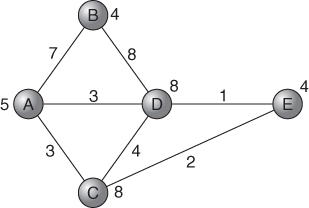
10.93 ![]()
10.94 ![]()
10.95 ![]()

We have clearly found a way of sharing the capital costs of the nodes among the arcs. Should any activity not be able to meet the capital cost demanded of it, it should be cut out. This allocation of capital costs will be such as to lead to the most profitable network. Using the numbers given on the network in Figure 10.3, the following shadow prices result as shown in Table 10.1.
| Constraint | Shadow Price |
| − δA + δAB ≤ 0 | 5 |
| − δB + δAB ≤ 0 | 2 |
| − δA + δAC ≤ 0 | 0 |
| − δC + δAC ≤ 0 | 3 |
| − δA + δAD ≤ 0 | 0 |
| − δD + δAD ≤ 0 | 3 |
| − δB + δBD ≤ 0 | 2 |
| − δD + δBD ≤ 0 | 6 |
| − δC + δCD ≤ 0 | 4 |
| − δD + δCD ≤ 0 | 0 |
| − δC + δCE ≤ 0 | 0 |
| − δE + δCE ≤ 0 | 2 |
| − δD + δDE ≤ 0 | 0 |
| − δE + δDE ≤ 0 | 1 |
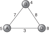
It will be seen that, for example, node C will receive 3 from AC, 4 from CD and 0 from CE. Clearly node C is no longer viable and must be cut. Applying similar arguments to all the other nodes, we are left with the optimal network shown in Figure 10.4.
An interesting observation following from duality in LP is that dividing up the capital costs of the nodes in other ways among the arcs could not lead to a more profitable network and could well lead to a less profitable one.
It should have become apparent from all the discussion in this section that there is no generally satisfactory way of getting the subsidiary economic information from an IP model that often proves so valuable in the case of LP. This topic represents a considerable gap in mathematical programming theory. The subject is more fully discussed in Williams (1979, 1997). Appa (1997) shows that after fixing the values of integer variables in a mixed integer programming model, the structural duality of the resulting LP model can sometimes be used. Greenberg (1998) gives a bibliography.
10.4 Sensitivity analysis and the stability of a model
We saw in Section 6.3 that having built and solved an LP model, it was very important to see how sensitive the answer was to changes in the data from which the model was constructed. Using ranging procedures on the objective and right-hand side coefficients, some insight into this could be obtained. In addition, it was shown how a model could, to some extent, be built in order to behave in a ‘stable’ fashion. Our considerations here are exactly the same as those in Section 6.3, only they concern IP models. As in the Section 10.3, we will see that IP models present considerable extra difficulties. This section falls into two parts. Firstly, we consider ways of testing the sensitivity of the solution of an IP model. Secondly, we consider how models may be built in order that they may exhibit stability.
10.4.1 Sensitivity analysis and integer programming
A theoretical way of doing sensitivity analysis on the objective coefficients of a model would be to replace the constraints by constraints representing the convex hull of feasible integer points. The model could then be treated as an LP model and objective ranging performed as described in Section 6.3.
For those PIP models where a reformulation easily yields the constraints for the convex hull, this is fairly straightforward. Otherwise, it is not a practical way of approaching the problem. Nor does it give a way of performing right-hand side ranging.
For MIP models solved by the branch and bound method, a sensitivity analysis can be performed on the LP sub-problem at the node giving the optimal integer solution. Alternatively, the integer variables can be fixed at their optimal values and a sensitivity analysis performed on the continuous part of the problem. These approaches clearly have the same drawbacks as those apparent when using similar approaches to derive economic information from an IP model as described in Section 10.3.
The only really satisfactory method of sensitivity analysis in IP involves solving the model again with changed coefficients and comparing optimal solutions. Obviously, the subsequent time to solve the model should be able to be reduced by exploiting the knowledge of the previous solution.
10.4.2 Building a stable model
In an LP model, the optimal value of the objective function varies continuously as the right-hand side and objective coefficients are changed. In an IP model, this may not happen. We consider the following very simple example.
The optimal value of the objective function is obviously not a continuous function of the right-hand side coefficient. In many practical situations, this is unrealistic. Suppose constraint (10.97) represented a budgetary limitation and the 0–1 variables referred to capital investments. It is very unlikely that a small decrease in the budget would cause us radically to alter our plans. A more likely occurrence is that the budget would be stretched slightly at some increased cost or the cost of one of the capital investments would be trimmed slightly. It is important that if this is the case this should be represented in the model. As it stands, the above example represents a poor model of the situation.
One way to remodel constraint (10.97) is to use the device described in Section 3.3 in order to allow constraints to be violated at a certain cost. A surplus (continuous) variable u is added into constraint (10.97) and given a cost (say 20) in the objective. This results in the following model:
10.98 ![]()
For a right-hand side of 16, the optimal solution is still δ1 = δ2 = 1, giving an objective value of 75.
If the right-hand side value of 16 is reduced slightly, the effect of u will be to ‘top the budget up’ to 16 at a unit cost of 20. For example, if the right-hand side falls to ![]() , u will become
, u will become ![]() We will retain the same optimal solution but the objective will fall by 10 to 65. As the right-hand side is further reduced, the optimal value of the objective will continue gradually to fall until we reach a right-hand side value of
We will retain the same optimal solution but the objective will fall by 10 to 65. As the right-hand side is further reduced, the optimal value of the objective will continue gradually to fall until we reach a right-hand side value of ![]() . We will then have the solution δ1 = 1, δ4 = 1 and δ5 = 1 as an alternative optimum. If the right-hand side is further reduced, we will transfer to this alternative optimum. It can be seen that this device of adding a surplus variable to the problem with a certain cost has two desirable effects on the model:
. We will then have the solution δ1 = 1, δ4 = 1 and δ5 = 1 as an alternative optimum. If the right-hand side is further reduced, we will transfer to this alternative optimum. It can be seen that this device of adding a surplus variable to the problem with a certain cost has two desirable effects on the model:
In some applications, we might wish to add a slack (continuous) variable v as well; giving v a cost in the objective (of say 8). This would result in the following model:
10.99 ![]()
This topic is not pursued further here as it has been fully covered for LP problems in Section 6.3. It is important to notice, however, the desirability of forcing the optimal solution of an IP model to vary ‘continuously’ with the data coefficients. Clearly, for many logical type constraints which appear in MIP models, it is meaningless to use a device such as that above. There are some classes of MIP models where the continuity property can be shown to hold without further reformulation. This subject is discussed in greater depth by A. C. Williams (1989).
10.5 When and how to use integer programming
In this section we try, very briefly, to summarize some of the points made in the preceding three chapters as a quick guide to using IP.
Finally, it should be pointed out that theoretical and computational progress in IP is being made all the time, making it possible to solve larger and more complex models.