Chapter 14
Solutions to problems
Optimal solutions to the problems presented in Part II are given here. The main purpose in giving the solutions is to allow the reader to check solutions he/she may have obtained to the same problems. All the solutions given here result from the formulations presented in Part III. Sometimes, alternative optimal solutions are possible, as described in Section 6.2, although the optimal value of the objective function will be unique.
If the reader obtains a different solution to a problem from that given here, he/she should attempt to validate his/her solution using the principles described in Section 6.1. In many cases, it is realistic to take the solution given here to represent the current operating pattern in the situation being modelled. The different solution obtained can then be validated relative to this solution.
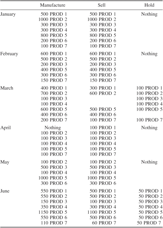
14.1 Food manufacture 1
The optimal policy is given in Table 14.1.
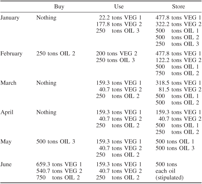
The profit (income from sales − cost of raw oils) derived from this policy is £107 843. This figure includes storage costs for the last month.
There are alternative optimal solutions.
14.2 Food manufacture 2
This model proved comparatively hard to solve. The optimal solution found is given in Table 14.2.
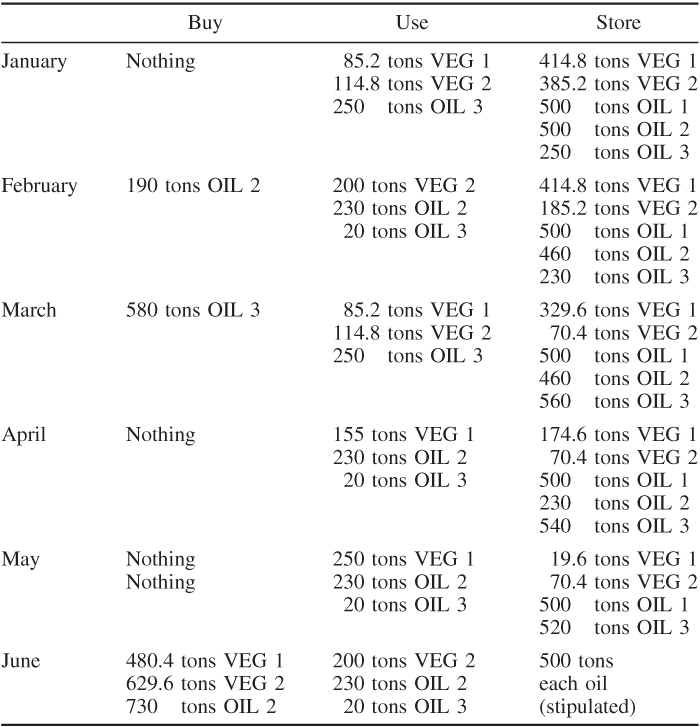
The profit (income from sales − cost of raw oils) derived from this policy is £100 279. There are alternative, equally good, solutions. This solution was obtained after 645 nodes. A total of 2007 nodes were examined to prove optimality.
14.3 Factory planning 1
The optimal policy is given in Table 14.3.
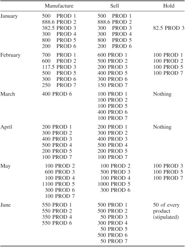
This policy yields a total profit of £93 715.
Information on the value of acquiring new machines can be obtained from the shadow prices on the appropriate constraints. The value of an extra hour in the particular month when a particular type of machine is used to capacity is given below:
| Machines used to capacity | Value | |
| January | Grinders | £8.57 |
| February | Horizontal drills | £0.625 |
| March | Borer | £200a |
a The borer is not in use in March. This figure indicates the high value of putting it into use. As explained in Section 6.2, these figures only give the marginal value of increases in capacity and can only therefore be used as indicators.
14.4 Factory planning 2
There are a number of alternative optimal maintenance schedules. One such is to put the following machines down for maintenance in the following months:
| January | — |
| February | One vertical drill, one horizontal drill |
| March | One grinder, two horizontal drills |
| April | One grinder, one borer, one planer |
| May | One vertical drill |
| June | — |
This results in the production and marketing plans are shown in Table 14.4.
These plans yield a total profit of £108 855.
There is, therefore, a gain of £15 140 over the six months by seeking an optimal maintenance schedule instead of the one imposed in the FACTORY PLANNING solution.
This solution was obtained in 191 nodes. The optimal objective value of £93 715 for the factory planning solution can be used as an objective cut-off because this clearly corresponds to a known integer solution. A total of 3320 nodes were needed to prove optimality.
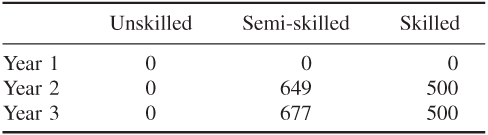
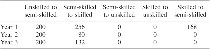
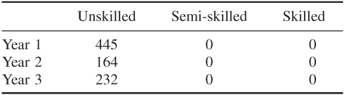
14.5 Manpower planning
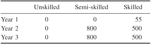
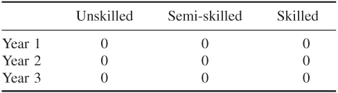
With the objective of minimizing redundancy, the optimal policies to pursue are given below:
Recruitment
Retraining and downgrading
Redundancy
Short-time working

Overmanning
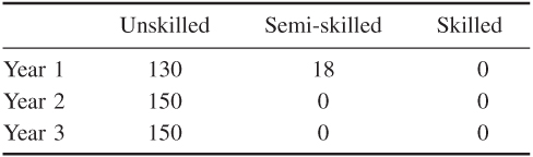
These policies result in a total redundancy of 842 workers over the three years. The total cost of pursuing these policies is £1 438 383.
In order to obtain this total cost, it is important to recognize that there are alternative solutions and we should choose that with minimum cost.
If the objective is to minimize the cost, the optimal policies are those given below:
Recruitment
Retraining and downgrading

Redundancy
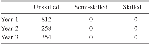
Short-time working
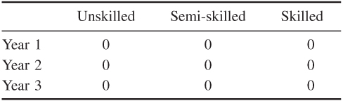
Overmanning
These policies cost £498 677 over the three years and result in a total redundancy of 1424 workers. Again, alternative solutions should be considered if necessary to ensure that this redundancy is the minimum possible for this (minimum) level of cost.
Clearly, minimizing costs instead of redundancy saves £939 706 but results in 582 extra redundancies.
The cost of saving each job (when minimizing redundancy) could, therefore, be regarded as £1615.
14.6 Refinery optimization
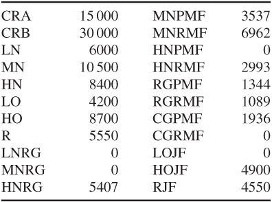
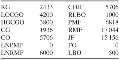
The optimal solution results in a profit of £211 365.
The optimal values of the variables defined in Part III are given below:
14.7 Mining
The optimal solution is as follows: work the following mines in each year
| Year 1 | Mines 1, 3, 4 |
| Year 2 | Mines 2, 3, 4 |
| Year 3 | Mines 1, 3 |
| Year 4 | Mines 1, 2, 4 |
| Year 5 | Mines 1, 2, 3 |
Keep every mine open each year apart from mine 4 in year 5.
Produce the following quantities of ore (in millions of tons) from each mine every year: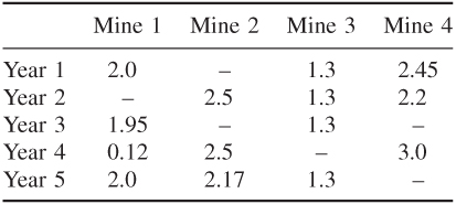
Produce the following quantities of blended ore (in millions of tons) each year:
| Year 1 | 5.75 |
| Year 2 | 6.00 |
| Year 3 | 3.25 |
| Year 4 | 5.62 |
| Year 5 | 5.47 |
This solution results in a total profit of £146.84 millions.
14.8 Farm planning
The optimal plan results in a total profit of £121 719 over the five years. Each year's detailed plan should be as follows:
| Year 1 | Grow 22 tons of grain on group 1 land |
| Grow 91 tons of sugar beet | |
| Buy 37 tons of grain | |
| Sell 23 tons of sugar beet | |
| Sell 31 heifers (leaving 23) |
The profit on the year will be £21 906.
| Year 2 | Grow 22 tons of grain on group 1 land |
| Grow 94 tons of sugar beet | |
| Buy 35 tons of grain | |
| Sell 27 tons of sugar beet | |
| Sell 41 heifers (leaving 12) |
The profit on the year will be £21 888.
| Year 3 | Grow 22 tons of grain on group 1 land |
| Grow 3 tons of grain on group 2 land | |
| Grow 98 tons of sugar beet | |
| Buy 38 tons of grain | |
| Sell 25 tons of sugar beet | |
| Sell 57 heifers (leaving none) |
The profit on the year will be £25 816.
| Year 4 | Grow 22 tons of grain on group 1 land |
| Grow 115 tons of sugar beet | |
| Buy 40 tons of grain | |
| Sell 42 tons of sugar beet | |
| Sell 57 heifers (leaving none) |
The profit on the year will be £26 826.
| Year 5 | Grow 22 tons of grain on group 1 land |
| Grow 131 tons of sugar beet | |
| Buy 33 tons of grain | |
| Sell 67 tons of sugar beet | |
| Sell 51 heifers (leaving none) |
The profit on the year will be £25 283.
Only in year 1, the accommodation limits the total number of cows. No investment should be made in further accommodation.
At the end of the five-year period, there will be 92 dairy cows.
As pointed out in Part III, the numbers of cows of successively increasing ages in successive years are effectively fixed by the continuity constraints. This allows the model to be reduced using the procedures mentioned in Section 3.4. When this is done, a further 18 variables can be fixed (besides the 20 in the original model) and 38 constraints can be removed.
14.9 Economic planning
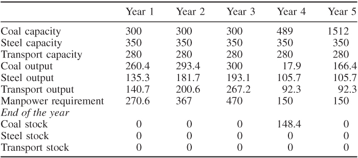
With the first objective (maximizing total productive capacity in year 5), the growth pattern shown in Table 14.5 results in a total productive capacity of £2142 million in year 5. Quantities are in million pounds.
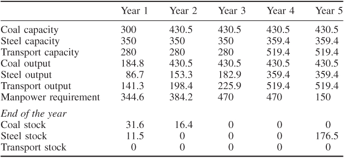
With the second objective (maximizing total production in the fourth and fifth years), the growth pattern shown in Table 14.6 results in a total output of £2619 millions in those years.
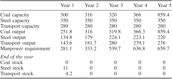
With the third objective (maximizing manpower requirements), the growth pattern shown in Table 14.7 results in a total manpower usage of £2450 millions.
The first objective obviously results in effort being concentrated on building up capacity in the coal industry. This happens because the production of extra coal capacity uses comparatively little output from the other industries.
With the second objective, more effort is put onto the transport industry. This results, in part, from the fact that transport uses less manpower than other industries.
With the third objective, the coal industry is again boosted in view of its heavy manpower requirement.
14.10 Decentralization
The optimal solution is
This results in a yearly benefit of £80 000 but communications costs of £65 100. It is interesting to note that communication costs are also reduced by moving out of London in this problem because they would have been £78 000 if each department had remained in London.
The net yearly benefit (benefits less communication costs) is therefore £14 900.
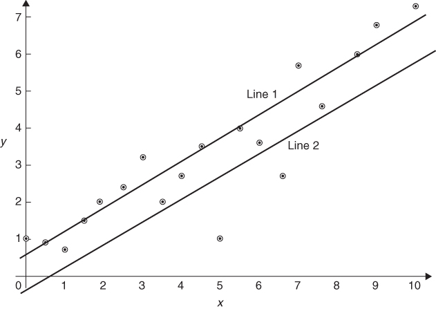
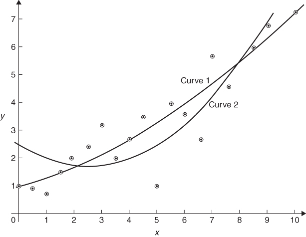
14.11 Curve fitting
![]()
![]()
![]()
![]()
A way of obtaining analytical solutions to these sorts of problems is described by Williams and Munford (1999).
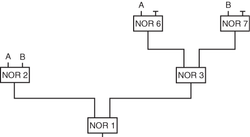
14.12 Logical design
The optimal solution is shown in Figure 14.3. There are, of course, symmetric alternatives.
14.13 Market sharing
This model proves difficult to solve optimally although a feasible solution is comparatively easy to obtain. Using the original formulation with no extra constraints, a feasible solution was found after 21 nodes by minimizing the sum of percentage deviations. This solution gave a sum of percentage deviations of 8.49 with the maximum such deviation being 3.73% (the Region 3 OIL goal). The best solution obtained in this run was after 360 nodes with a sum of percentage deviations of 4.53, the maximum such deviation being 2.5% (the DELIVERY POINTS goal). After a total of 1995 nodes, the search was completed.
Minimizing the maximum percentage deviation produced a feasible solution after 37 nodes. This solution gave a maximum deviation of 2.5% (the OIL in region 3 goal). The sum of percentage deviations was 8.82. This was proved to be the optimal solution after 3158 nodes.
The second formulation was obtained by adding 228 ‘facets’ for the OIL goals in the three regions. The increased size of this model drastically reduced the number of nodes that could be explored in a given time. After 10 s with the objective of minimizing the sum of percentage deviations, 75 nodes had been explored with a minimum sum of percentage deviations of 11.28 obtained at node 61. The maximum deviation associated with this solution was 2.77% (the SPIRITS goal). When the objective was to minimize the maximum deviation, 36 nodes were explored with no feasible solution being found.
The most successful formulation was the third one, where six single ‘tighter’ constraints, logically equivalent to the six constraints implied by the OIL goals in the three regions, were added. With the objective of minimizing the sum of percentage deviations, a feasible solution was obtained after 35 nodes. The sum of percentage deviations was 8.83, and the maximum deviation was 2.5% (in the GROWTH prospects goals). This run was terminated after 394 nodes with no other feasible solutions being found.
With the objective of minimizing the maximum deviation, a feasible solution was found after 44 nodes with a maximum deviation of 3.15% (in the SPIRITS goal). The associated sum of percentage deviations was 12.14. A better solution was found at node 200 with a maximum deviation of 2.5% (in the GROWTH prospects goals). The associated sum of percentage deviations was 9.7. No better solutions were found after 303 nodes.
With hindsight, it is possible to observe that the minimax objective cannot be reduced below 2.5% because the slack variable in the GROWTH goal cannot be less than 0.2, given a right-hand side of 3.2. Therefore, the slack in this constraint was fixed at 0.2 and the surplus at 0. The third formulation of the problem was then rerun in order to minimize the sum of percentage deviations. At node 681, the optimal integer solution was found where the sum of percentage deviations was 7.806. The solution was proved optimal after 889 nodes. This optimal solution allocates the following retailers to D1:
![]()
All other retailers are to be assigned to division D2.
This problem has proved of considerable interest in view of its computational difficulty. A remodelling approach using ‘basis reduction’ is described by Aardal et al. (1999).
14.14 Opencast mining
The optimal solution is to extract the shaded blocks shown in Figure 14.4. This results in a profit of £17 500.
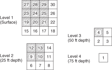
This solution was obtained in 28 iterations.
14.15 Tariff rates (power generation)
The following generators should be working in each period giving the following outputs:
| Period 1 | 12 of type 1, output 10 200 MW |
| 3 of type 2, output 4 800 MW | |
| Period 2 | 12 of type 1, output 16 000 MW |
| 8 of type 2, output 14 000 MW | |
| Period 3 | 12 of type 1, output 11 000 MW |
| 8 of type 2, output 14 000 MW | |
| Period 4 | 12 of type 1, output 21 250 MW |
| 9 of type 2, output 15 750 MW | |
| 2 of type 3, output 3 000 MW | |
| Period 5 | 12 of type 1, output 11 250 MW |
| 9 of type 2, output 15 750 MW |
The total daily cost of this operating pattern is £988 540.
Deriving the marginal cost of production from a mixed integer programming model such as this encounters the difficulties discussed in Section 10.3. We could adopt the approach of fixing the integer variables at the optimal integer values and obtaining this economic information from the resulting linear programming model. The marginal costs then result from any changes within the optimal operating pattern, that is, without altering the numbers of different types of generator working in each period (although their levels of operation could vary).
The marginal costs of production per hour are then obtained from the shadow prices on the demand constraints (divided by the number of hours in the period). These give:
| Period 1 | £1.3 per megawatt hour |
| Period 2 | £2 per megawatt hour |
| Period 3 | £2 per megawatt hour |
| Period 4 | £2 per megawatt hour |
| Period 5 | £2 per megawatt hour |
With this method of obtaining marginal valuations, there will clearly be no values associated with the reserve output guarantee constraints because all the variables have been fixed in these constraints.
As an alternative to using the above method of obtaining marginal valuations on the constraints, we could take the shadow prices corresponding to the continuous optimal solution. In this model, this solution (the continuous optimum) does not differ radically from the integer optimum. It gives the following operating pattern that is clearly unacceptable in practice because of the fractional number of generators working:
| Period 1 | 12 of type 1, | output 10 200 MW |
| 2.75 of type 2, | output 4 800 MW | |
| Period 2 | 12 of type 1, | output 15 200 MW |
| 8.46 of type 2, | output 14 800 MW | |
| Period 3 | 12 of type 1, | output 10 200 MW |
| 8.46 of type 2, | output 14 800 MW | |
| Period 4 | 12 of type 1, | output 21 250 MW |
| 9.6 of type 2, | output 16 800 MW | |
| 1.3 of type 3, | output 1 950 MW | |
| Period 5 | 12 of type 1, | output 10 200 MW |
| 9.6 of type 2, | output 16 800 MW |
The resulting objective value (cost) is £985 164.
The shadow prices on the demand constraints imply the following marginal costs of production:
| Period 1 | £1.76 per megawatt hour |
| Period 2 | £2 per megawatt hour |
| Period 3 | £1.79 per megawatt hour |
| Period 4 | £2 per megawatt hour |
| Period 5 | £1.86 per megawatt hour |
In this case, we can obtain a meaningful valuation for the 15% reserve output guarantee from the shadow prices on the appropriate constraints. The only non-zero valuation is on the constraint for period 4. This indicates that the cost of each guaranteed hour is £0.042. The range on the right-hand side coefficient of this constraint indicates that the 15% output guarantee can change between 2% and 52% with the marginal cost of each extra hour being £0.042.
14.16 Hydro power
The following thermal generators should be working in each period, giving the following outputs:
| Period 1 | 12 of type 1, | output 10 565 MW |
| 3 of type 2, | output 5 250 MW | |
| Period 2 | 12 of type 1, | output 14 250 MW |
| 9 of type 2, | output 15 750 MW | |
| Period 3 | 12 of type 1, | output 10 200 MW |
| 9 of type 2, | output 15 750 MW | |
| Period 4 | 12 of type 1, | output 21 350 MW |
| 9 of type 2, | output 15 750 MW | |
| 1 of type 3, | output 1 500 MW | |
| Period 5 | 12 of type 1, | output 10 200 MW |
| 9 of type 2, | output 15 750 MW |
The only hydro generator to work is B in periods 4 and 5, producing an output of 1400 MW.
Pumping should take place in the following periods at the given levels:
| Period 1 | 815 MW |
| Period 3 | 950 MW |
| Period 5 | 350 MW |
Although it may seem paradoxical to both pump and run Hydro B in period 5, this is necessary to meet the requirement of the reservoir being at 16 m at the beginning of period 1, given that the Hydro can work only at a fixed level. It would be possible to use the model to cost this environmental requirement.
The height of the reservoir at the beginning of each period should be
| Period 1 | 12 m |
| Period 2 | 17.63 m |
| Period 3 | 17.63 m |
| Period 4 | 19.53 m |
| Period 5 | 18.12 m |
The cost of these operations is £986 630.
In solving this model, it is valuable to exploit the fact that the optimal objective value must be less than or equal to that reported in Section 14.15. This is for two reasons. First, the optimal solution in Section 14.15 using only thermal generators is a feasible solution to this model. Second, the 15% extra output guarantee can be met at no start-up cost using the hydro generators. When solving this model by the branch-and-bound method, the optimal objective value in Section 14.15 could be used as an ‘objective cut-off’ to prune the tree search.
Planning the use of hydro power by means of Stochastic Programming in order to model uncertainty is described by Archibald et al. (1999).
14.17 Three-dimensional noughts and crosses
The minimum number of lines of the same colour is four. There are many alternative solutions, one of which is given in Figure 14.5, where the top, middle and bottom sections of the cube are given. Cells with black balls are shaded.
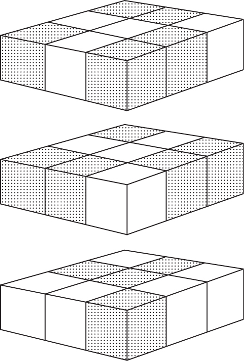
This solution was obtained in 15 nodes. A total of 1367 nodes were needed to prove optimality.
14.18 Optimizing a constraint
The ‘simplest’ version of this constraint (with minimum right-hand side coefficient) is
![]()
This is also the equivalent constraint with the minimum sum of absolute values of the coefficients.
14.19 Distribution 1
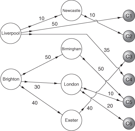
The minimum cost distribution pattern is shown in Figure 14.6 (with quantities in thousands of tons).

There is an alternative optimal solution in which the 40 000 ton from Brighton to Exeter comes from Liverpool instead.
This distribution pattern costs £198 500 per month.
Depot capacity is exhausted at Birmingham and Exeter. The value (in reducing distribution costs) of an extra ton per month capacity in these depots is £0.20 and £0.30, respectively.
This distribution pattern will remain the same as long as the unit distribution costs remain within certain ranges. These are given below (for routes which are to be used):
| Route | Cost range |
| Liverpool to C1 | −∞ to 1.5 |
| Liverpool to C6 | −∞ to 1.2 |
| Brighton to Birmingham | −∞ to 0.5 |
| Brighton to London | 0.3 to 0.8 |
| Brighton to Exeter | −∞ to 0.2 |
| Birmingham to C2 | −∞ to 1.2 |
| Birmingham to C4 | −∞ to 1.2 |
| Birmingham to C5 | 0.3 to 0.7 |
| London to C5 | 0.3 to 0.8 |
| Exeter to C3 | 0 to 0.5 |
Depot capacities can be altered within certain limits. For the not fully utilized depots of Newcastle and London changing capacity within these limits has no effect on the optimal distribution pattern. For Birmingham and Exeter the effect on total cost will be £0.2 and £0.3 per ton per month within the limits. Outside certain limits the prediction of the effect requires resolving the problem. The limits are:
| Depot | Capacity range |
| Birmingham | 45 000–105 000 tons |
| Exeter | 40 000–95 000 tons |
N.B. All the above effects of changes are only valid if one thing is changed at a time within the permitted ranges. Clearly, the above solution does not satisfy the customer preferences for suppliers.
By minimizing the second objective, it is possible to reduce the number of goods sent by non-preferred suppliers to a customer to a minimum. This was done and revealed that it is impossible to satisfy all preferences. The best that could be done resulted in the distribution pattern shown in Figure 14.7, where customer C5 receives 10 000 tons from his non-preferred depot of London. This is the minimum cost such distribution pattern. (There are alternative patterns which also minimize the number of non-preferences but which cost more.) The minimum cost here is £246 000, showing that the extra cost of satisfying more customers preferences is £47 500.
14.20 Depot location (distribution 2)
The minimum cost solution is to close down the Newcastle depot and open a depot in Northampton. The Birmingham depot should be expanded. The total monthly cost (taking account of the saving from closing down Newcastle) resulting from these changes and the new distribution pattern is £174 000. Figure 14.8 shows the new distribution pattern (with quantities in thousands of tons).
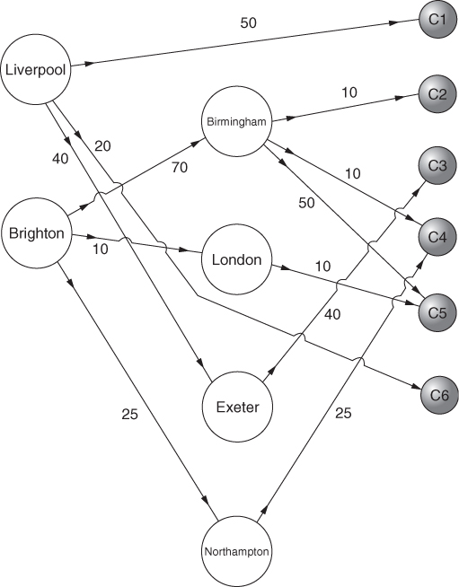
This solution was obtained in 40 iterations. The continuous optimal solution was integer. Therefore, no tree search was necessary.
14.21 Agricultural pricing
The optimal prices are:
| Milk | £303 per ton |
| Butter | £667 per ton |
| Cheese 1 | £900 per ton |
| Cheese 2 | £1085 per ton |
The resultant yearly revenue will be £1992 million. It is straightforward to calculate the yearly demands that will result from these prices. They are:
| Milk | 4 781 000 tons |
| Butter | 384 000 tons |
| Cheese 1 | 250 000 tons |
| Cheese 2 | 57 000 tons |
The economic cost of imposing a constraint on the price index can be obtained from the shadow price on the constraint. For this example, this shadow price in the optimal solution indicates that each £1 by which the new prices are allowed to increase the cost of past year's consumption would result in an increased revenue of £0.61.
14.22 Efficiency analysis
The efficient garages turn out to be 3 (Basingstoke), 6 (Newbury), 7 (Portsmouth), 8 (Alresford), 9 (Salisbury), 11 (Alton), 15 (Weymouth), 16 (Portland), 18 (Petersfield), 22 (Southampton), 23 (Bournemouth), 24 (Henley), 25 (Maidenhead), 26 (Fareham) and 27 (Romsey).
It should be observed that these garages may be efficient for different reasons. For example, Newbury has 12 times the staff of Basingstoke but only five times as much showroom space. It sells 10 times as many Alphas and 10.4 times as many Betas and makes nine times as much profit. This suggests that it makes more efficient use of showroom space but less of staff.
The other garages are deemed inefficient. They are listed in Table 14.8 in decreasing order of efficiency together with the multiples of the efficient garages that demonstrate them to be inefficient.
| Garage | Efficiency number | Multiples of efficient garages |
| 19 Petworth | 0.988 | 0.066(6) + 0.015(18) + 0.034(25) + 0.675(26) |
| 21 Reading | 0.982 | 1.269(3) + 0.544(15) + 1.199(16) + 2.86(24) |
| + 1.37(25) | ||
| 14 Bridport | 0.971 | 0.033(3) + 0.470(16) + 0. 783(24) + 0.195(25) |
| 2 Andover | 0.917 | 0.857(15) + 0.215(25) |
| 28 Ringwood | 0.876 | 0.008(3) + 0.320(16) + 0.146(24) |
| 5 Woking | 0.867 | 0.952(8) + 0.021(11) + 0.009(22) + 0.148(25) |
| 4 Poole | 0.862 | 0.329(3) + 0.757(16) + 0.434(24) + 0.345(25) |
| 12 Weybridge | 0.854 | 0.797(15) + 0.145(25) + 0.018(26) |
| 1 Winchester | 0.840 | 0.005(7) + 0.416(8) + 0.403(9) + 0.333(15) |
| + 0.096(16) | ||
| 13 Dorchester | 0.839 | 0.134(3) + 0.104(8) + 0.119(15) + 0.752(16) |
| + 0.035(24) + 0.479(26) | ||
| 20 Midhurst | 0.829 | 0.059(9) + 0.066(15) + 0.472(16) + 0.043(18) |
| + 0.009(25) | ||
| 17 Chichester | 0.824 | 0.058(3) + 0.097(8) + 0.335(15) + 0.166(16) |
| + 0.236(24) + 0.154(26) | ||
| 10 Guildford | 0.814 | 0.425(3) + 0.150(7) + 0.623(8) + 0.192(15) |
| + 0.168(16) |
For example, the comparators to Petworth taken in the multiples given below use inputs of:
| Staff | 5.02 |
| Showroom space | 550 m2 |
| Category 1 population | 2 (1000s) |
| Category 2 population | 2 (1000s) |
| Alpha enquiries | 7.35 (100s) |
| Beta enquiries | 3.98 (100s) |
to produce outputs of:
| 1.518 (1000s) | Alpha sales |
| 0.568 (1000s) | Beta sales |
| 1.568 (million pounds) | Profit |
Clearly, this uses no more than the inputs used by Petworth but produces outputs at least 1.0119 times as great.
There is also a useful interpretation of the dual values on the input and output constraints. These can be regarded as weightings that the particular garage would like to place on its inputs and outputs so as to maximize this weighted ratio of outputs to inputs but keep the corresponding ratios for the other garages above 1 (i.e. not allow them to appear inefficient). In the case of Petworth, the dual values from solving the model turn out to be 0, 0.1557, 0.0618, 0.0158, 0 and 0 for the inputs and 0.1551, 0 and 0.495 for the outputs.
This gives a weighted ratio of
![]()
This is clearly the efficiency number. Petworth weighs most heavily high outputs that bring it out in the best light and least heavily high inputs.
The dual formulation referred to in Sections 3.2 and 13.22 chooses the weights so as to maximize this ratio while not allowing the ratios for other garages (with these weights) to fall below 1.
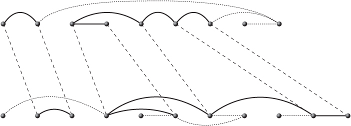
14.23 Milk collection
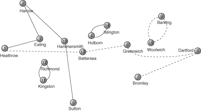
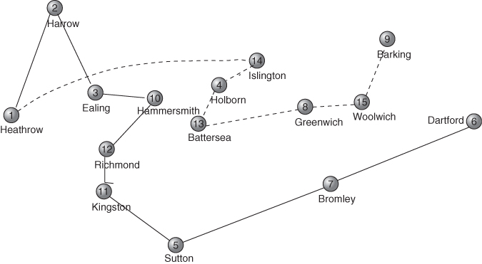
The optimal solution is given in Figure 14.9 with dashes representing the first day's routes and dotted lines those of the second day. The total distance covered is 1229 miles.
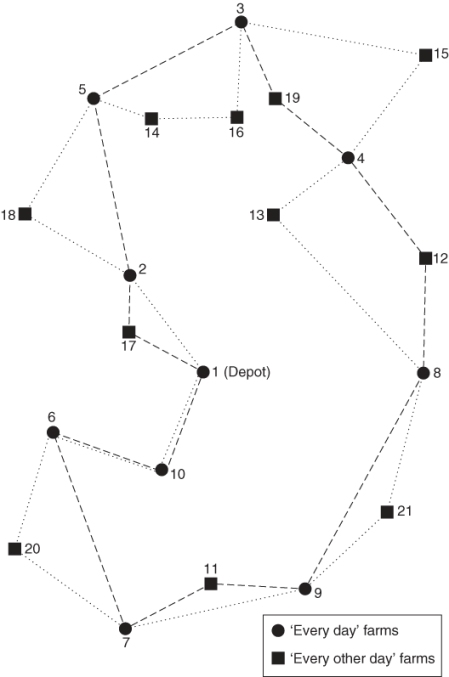
In the formulation given in Section 13.23, this first solution produced subtours on day 1 around farms 2, 5 and 18; around 3, 16, 13, 4 and 19 and around 1, 8, 21, 9, 11, 7, 6 and 10 and on day 2, around farms 6, 7 and 20 and around all the other farms. This infeasible solution covers 1214 miles (there are alternative, equally good solutions). Subtour elimination constraints were then introduced to prevent the subtours (on both days to prevent them re-arising on the other day), resulting in another solution with no subtours on day 1 but subtours on day 2 around farms 1, 2, 17, 6, 7 and 10; around 4, 15, 3, 5, 14, 16 and 13 and around 8, 9 and 21. Subtour elimination constraints were introduced to prevent these subtours (on both days). This resulted in the optimal solution (no subtours) given in Figure 14.9.
These stages required 34, 13 and 272 nodes, respectively. Out of interest, not introducing the ‘disaggregated’ constraints described in Section 13.23 resulted in the first stage taking 1707 nodes.
This problem is based on a larger one described by Butler, Williams and Yarrow (1997). That larger problem required a more sophisticated solution approach using generalizations of known results concerning the structure of the travelling salesman polytope.
14.24 Yield management
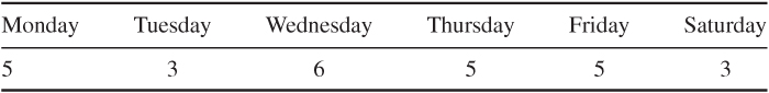
Numbers of seats have been rounded to nearest integers where necessary.
Period 1
Sell tickets at the following prices up to what is available:
| First | £1200 |
| Business | £900 |
| Economy | £500 |
Set provisional prices for period 2:
| First | £1150 if scenario 1 in period 1 |
| £1150 if scenario 2 in period 1 | |
| £1300 if scenario 3 in period 1 | |
| Business | £1100 for all scenarios in period 1 |
| Economy | £700 for all scenarios in period 1 |
Set provisional prices for period 3:
| First | £1500 for all scenarios in periods 1 and 2 |
| Business | £800 for all scenarios in periods 1 and 2 |
| Economy | £480 for all scenarios in period 1 and scenarios 1 and 2 in period 2; £450 for all scenarios in period 1 and scenario 3 in period 2 |
(Provisionally) book three planes. Expected revenue is £169 544.
Period 2
Rerunning the model with the demand given (with hindsight) for the price levels decided for period 1 results in the following recommended decisions for period 2.
Sell tickets at the following prices up to what is available:
| First | £1150 |
| Business | £1100 |
| Economy | £700 |
Set provisional prices for period 3:
| First | £1500 for all scenarios in period 2 |
| Business | £800 for all scenarios in period 2 |
| Economy | £480 for scenarios 1 and 2 in period 2 |
| £450 for scenario 3 in period 2 |
(Provisionally) still book three planes. Expected total revenue is now £172 969.
Period 3
Rerunning the model with the known demands and price levels for periods 1 and 2 results in the following recommended decisions for period 3.
Sell tickets at the following prices up to what is available:
| First | £1500 |
| Business | £800 |
| Economy | £480 |
(Provisionally) still book three planes. Expected total revenue is now £176 392.
Solution
The resultant solution at take-off (using demands during the final week) will therefore be:
Period 1
| First Class | 25 seats sold at £1200: Yield £30 000 |
| Business Class | 45 seats sold at £900: Yield £40 500 |
| Economy Class | 50 seats sold at £500: Yield £25 000 |
Period 2
| First Class | 50 seats sold at £1150: Yield £57 500 |
| Business Class | 45 seats sold at £1100: Yield £49 500 |
| Economy Class | 50 seats sold at £700: Yield £35 000 |
Period 3
| First Class | 40 seats sold at £1500: Yield £60 000 |
| Business Class | 25 seats sold at £800: Yield £20 000 |
| Economy Class | 36 seats sold at £480: Yield £17 280 |
Three planes will be needed. Total yield (subtracting the costs of the planes) will therefore be £184 780.
It will be necessary to reallocate four seats from Business to First Class and five seats from Economy to Business Class.
If the model is altered to maximize yield subject to expected demand (without recourse), the resultant solution (allowing for the given demands falling below those expected) is:
Period 1
| First Class | 24 seats sold at £1200: Yield £28 800 |
| Business Class | 39 seats sold at £900: Yield £35 100 |
| Economy Class | 50 seats sold at £500: Yield £25 000 |
Period 2
| First Class | 55 seats sold at £1150: Yield £63 250 |
| Business Class | 43 seats sold at £1100: Yield £47 300 |
| Economy Class | 49 seats sold at £700: Yield £34 300 |
Period 3
| First Class | 34 seats sold at £0.1500: Yield £51 000 |
| Business Class | 35 seats sold at £800: Yield £28 000 |
| Economy Class | 37 seats sold at £480: Yield £17 760 |
Three planes are needed. Total yield is £180 210.
This can clearly be improved by, in the last period, ‘topping-up’ to fill vacant capacity in the most beneficial way, that is, selling 39 Economy Class instead of 37, so filling the three planes.
This increases yield to £181 170, which is still considerably short of the yield produced by running the Stochastic Program with recourse.
14.25 Car rental
The numbers of cars in all aspects of the following solution have been rounded from the fractional answers that result from the linear programming model.
The company should own 624 cars and pursue the following policies that will result in a weekly profit of £122 398.
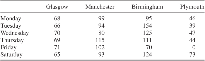
The estimated number of undamaged cars in each depot at the beginning of each day will be as follows (there will also be hired out cars not in any depot).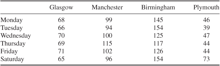
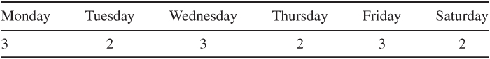
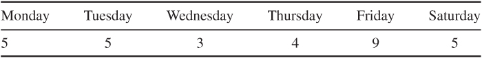
The estimated number of damaged cars in each depot at the beginning of each day will be as follows.
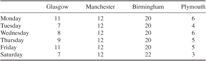
Of the undamaged cars, the following should be rented out each day, for the periods and destinations in the proportions given in the statement of the problem.
No transfers of undamaged cars should be made but the following transfers of damaged cars should be made (arriving the following day).
Glasgow to Manchester
Glasgow to Birmingham
Plymouth to Birmingham
The two repair depots of Manchester and Birmingham are fully occupied on all six days repairing 12 and 20 cars, respectively, each day. Repair capacity is clearly a limiting factor on the operation of the company. This is reflected by the high-shadow prices on the repair capacity constraints, which vary between £617 and £646 per car per day in both repairing depots. A plan to increase repair capacity forms the subject of problem 12.27. The solution above was obtained in 153 iterations.
14.26 Car rental 2
Only the Birmingham repair capacity should be increased, using both expansion options, to expand to 22 cars per day. Repair capacities in all depots are again fully used.
This allows the company to expand its fleet to 895 cars, resulting in a new weekly profit of £135 511. All demands still cannot be fully met.
This model solved in 5 nodes.
14.27 Lost baggage distribution
Two vans are needed. Solving the model, defined in Section 13.27 (a relaxation of the final model), leads to the ‘solution’ given in Figure 14.10. This required 2263 nodes to solve.
One van uses the bold lines and the other the dashed lines. Both take 120 min. Clearly, there are unacceptable subtours.
A total of 31 subtour elimination constraints needed to be appended, in 14 stages, in order to obtain a true solution with no subtours (there are a number of such solutions). This solution required 1296 nodes (a few seconds on a notepad computer). Fixing the number of vans needed at two and minimizing the maximum time needed by the vans took a further 561 nodes to solve (no additional subtour elimination constraints were needed). It produced the two routes illustrated in Figure 14.11, a bold line and a dashed line The times taken by the vans to reach their furthest locations are 99 and 100 min, respectively.
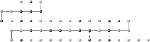
14.28 Protein folding
The model took 471 nodes to solve. Eight hydrophobic acids were matched (additional to those already contiguous) with folds between acids 3 and 4, 8 and 9, 22 and 23 and 35 and 36. The folded protein is illustrated in Figure 14.12 with the extra matches marked by dashed lines.
14.29 Protein comparison
This model took 253 branch-and-bound nodes to solve and resulted in the comparison illustrated in Figure 14.13 with five comparable edges demonstrating the lack of similarity between the two proteins.