Chapter 13

Formulation and discussion of problems

A suggested way of formulating each of the problems of Part II as a mathematical programming model is described. Each of these formulations is ‘good’ in the sense that it proved possible to solve the resultant model in a reasonable time on the computer system used. With some of the problems, other formulations were tried only to show that computation times were prohibitive. It must be emphasized that although the formulations presented here are the best known to the author, there are probably better formulations possible for some of the problems. Indeed, one of the purposes of the latter part of this book is to present concrete problems that may help advance the art of formulation.

All the models described here assume that a computer program is to be employed using one of the following algorithms:

These are the three algorithms that are most widely incorporated into commercial package programs.

For some of the problems, more specialized algorithms might be more efficient. In practice, the employment of such algorithms is often made difficult by the absence of efficient computer packages for handling large models. Where there is, however, obvious advantage to be gained from a specialized algorithm, this is pointed out in the discussion associated with the formulation description. This is particularly true where the model (or its dual) admits a network formulation. In such cases, it should still, however, be possible to solve the model reasonably efficiently using one of the above three methods. Sometimes, it is desirable to build a model in a particular way to suit a particular algorithm (particularly for integer programming problems). In the formulations here the models are all built on the assumption that one of the above three algorithms will be used.

Again, especially with integer programming models, it is often desirable to build a model with a particular branch and bound solution strategy in mind. When this is done the suggested strategy is explained.

Most of the models are very easy to solve. For the more difficult ones there is some computational discussion.

13.1 Food manufacture 1

Blending problems are frequently solved using linear programming. Linear programming has been used to find ‘minimum cost’ blends of fertilizer, metal alloys, clays and many food products, to name only a few. Applications are described in Fisher and Schruben (1953) and Williams and Redwood (1974), for example.

The problem presented here has two aspects. Firstly, it is a series of simple blending problems. Secondly, there is a purchasing and storing problem. To understand how this problem may be formulated, it is convenient to consider first the blending problem for only one month. This is the single-period problem that has already been presented as the second example in Section 1.2.

13.1.1 The single-period problem

If no storage of raw oils were allowed, the problem of what to buy and how to blend in January could be formulated as follows:

The variables x₁, x₂, x₃, x₄, x₅ represent the quantities of the raw oils that should be bought respectively, that is, VEG 1, VEG 2, OIL 1, OIL 2 and OIL 3. y represents the quantity of PROD that should be made.

The objective is to maximize profit, which represents the income derived from selling PROD minus the cost of the raw oils.

The first two constraints represent the limited production capacities for refining vegetable and non-vegetable oils.

The next two constraints force the hardness of PROD to lie between its upper limit of 6 and its lower limit of 3. It is important to model these restrictions correctly. A frequent mistake is to model them as

and

Such constraints are clearly dimensionally wrong. The expressions on the left have the dimension of hardness multiplied by quantity, whereas the figures on the right have the dimensions of hardness. Instead of the variables x_i in the above two inequalities, expressions x_i/y are needed to represent proportions of the ingredients rather than the absolute quantities x_i. When such replacements are made, the resultant inequalities can easily be re-expressed in a linear form as the constraints UHRD and LHRD.

Finally, it is necessary to make sure that the weight of the final product PROD is equal to the weight of the ingredients. This is done by the last constraint CONT, which imposes this continuity of weight.

The single-period problems for the other months would be similar to that for January apart from the objective coefficients representing the raw oil costs.

13.1.2 The multi-period problem

The decisions of how much to buy each month with a view to storing for use later can be incorporated into a linear programming model. To do this, a ‘multi-period’ model is built. It is necessary, each month, to distinguish the quantities of each raw oil bought, used and stored. These quantities must be represented by different variables. We suppose the quantities of VEG 1 bought, used and stored in each successive month are represented by variables with the following names:

BVEG 11,	BVEG 12,	and so on,
UVEG 11,	UVEG 12,	and so on,
SVEG 11,	SVEG 12,	and so on.

It is necessary to link these variables together by the relation

Initially (month 0) and finally (month 6), the quantities in store are constants (500). The relation above involving VEG 1 gives rise to the following constraints:

Similar constraints must be specified for the other four raw oils.

It may be more convenient to introduce variables SVEG 10, and so on, and SVEG 16, and so on, into the model and fix them at the value 500.

In the objective function, the ‘buying’ variables will be given the appropriate raw oil costs in each month. The storage variables will be given the cost of £5 (or ‘profit’ of –£5). Separate variables PROD 1, PROD 2, and so on, must be defined to represent the quantity of PROD to be made in each month. These variables will each have a profit of £150.

The resulting model will have the following dimensions as well as the single objective function:

6 × 5 =	30	buying variables
6 × 5 =	30	using variables
5 × 5 =	25	storing variables
		product variables
Total	91	variables

6 × 5 =	30	blending constraints (as in the single-period model)
6 × 5 =	30	storage linking constraints
Total	60	constraints

It is also important to realize the use to which a model such as this might be put for medium-term planning. By solving the model in January, buying and blending plans could be determined for January together with provisional plans for the succeeding months. In February, the model would probably be resolved with revised figures to give firm plans for February together with provisional plans for succeeding months up to and including July. By this means, the best use is made of the information for succeeding months to derive an operating policy for the current month.

13.2 Food manufacture 2

The extra restrictions stipulated are quite common in blending problems. It is often desired to (i) limit the number of ingredients in a blend; (ii) rule out small quantities of one ingredient and (iii) impose ‘logical conditions’ on the combinations of ingredients.

These restrictions cannot be modelled by conventional linear programming. Integer programming is the obvious way of imposing the extra restrictions. In order to do this, it is necessary to introduce 0–1 integer variables into the problem as described in Section 9.2. For each ‘using’ variable in the problem, a corresponding 0–1 variable is also introduced. This variable is used as an indicator of whether the corresponding ingredient appears in the blend or not. For example, corresponding to variable UVEG 11, a 0–1 variable DVEG 11 is introduced. These variables are linked together by two constraints. Supposing x₁ represents UVEG 11 and δ₁ represents DVEG 11, the following extra constraints are added to the model:

As δ₁ is only allowed to take the integer values 0 and 1, x₁ can only be non-zero (i.e. VEG 1 in the blend in month 1) if δ₁ = 1 and then it must be at a level of at least 20 tons. The constant 200 in the first of the above inequalities is a known upper limit to the level of UVEG 11 (the combined quantities of vegetable oils used in a month cannot exceed 200). Similar 0–1 variables and corresponding ‘linkage’ constraints are introduced for the other ingredients. Suppose x₂, x₃, x₄ and x₅ represent UVEG 21, UOIL 11; UOIL 21 and UOIL 31, then the following constraints and 0–1 variables are also introduced:

All these variables and constraints are repeated for all six months.

In this way, condition 2 in the statement of the problem is automatically imposed. Condition 1 can be imposed by the constraint

and the corresponding constraints for the other five months.

Condition 3 can be imposed in two possible ways: by the single constraints,

or by the pairs of constraints,

There is computational advantage to be gained by using the second pair of constraints as they are ‘tighter’ in the continuous problem (see Section 10.1). Similar constraints are, of course, imposed for the other five months.

The model has now been augmented in the following way:

6 × 5 =	30	0–1 variables
Total	30	extra variables (all integer)
2 × 6 × 5 =	60	linking constraints
	6	constraints for condition 1
2 × 6 =	12	constraints for condition 3
Total	78	extra constraints

It is also necessary to impose upper bounds of 1 on all the 30 integer variables.

There is probably advantage to be gained from the user specifying a priority order for the variables in order to control the tree search in the branch and bound algorithm. The six δ₅ variables (one for each month) were given priority in choosing branching variables.

13.3 Factory planning 1

This example is typical of some very common applications of linear programming. The objective is to find the optimum ‘product mix’ subject to the production capacity and the marketing limitations. As with the food manufacture problem, there are two aspects. Firstly, there is the single-period problem, then the extension to six months.

13.3.1 The single-period problem

If storage of finished products is not allowed, the model for January can be formulated as follows:

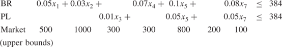
where GR, VD, HD, BR and PL stand for grinding, vertical drilling, horizontal drilling, boring and planing, respectively.

The variables x_i represent the quantities of PROD i to be made.

The single-period problems for the other months would be similar apart from different market bounds, and different capacity figures for the different types of machine.

13.3.2 The multi-period problem

It is necessary each month to distinguish the quantities of each product manufactured from the quantities sold and held over in storage. These quantities must be represented by different variables. Suppose the quantities of PROD 1 manufactured, sold and held over in successive months are represented by variables with the following names:

MPROD 11,	MPROD 12,	and so on,
SPROD 11,	SPROD 12,	and so on,
HPROD 11,	HPROD 12,	and so on.

It is necessary to link these variables together by the relation

Initially (month 0), there is nothing held but finally (month 6) there are 50 of each product held. This relation involving PROD 1 gives rise to the following constraints:

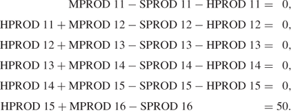
Similar constraints must be specified for the other six products.

It may be more convenient to define also variables HPROD 16, HPROD 26, and so on, and ‘fix’ them at the value 50.

In the objective function, the ‘selling’ variables are given the appropriate ‘unit profit’ figures and the ‘holding’ variables coefficients of −0.5.

The resulting model has the following dimensions:

6 × 7 = 42	manufacturing variables
6 × 7 = 42	selling variables
6 × 7 =	holding variables
Total 126	variables
6 × 5 = 30	capacity constraints
6 × 7 =	monthly linking constraints
Total 72	constraints

In addition, in each month, there are market bounds on the seven products and bounds on the holding quantities. This gives a total of 84 upper bounds.

13.4 Factory planning 2

The extra decisions that this problem requires over the factory planning problem requires the use of integer programming. This is a clear case of extending a linear programming model by adding integer variables with extra constraints.

It is convenient to number the different types of machine as below:

Type 1	Grinders
Type 2	Vertical drills
Type 3	Horizontal drills
Type 4	Borer
Type 5	Planer

13.4.1 Extra variables

Integer variables γ_it are introduced with the following interpretations:

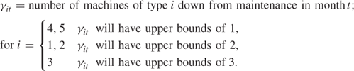
There are 30 such integer variables.

13.4.2 Revised constraints

The machining capacity constraints in the original model must be changed as capacity will now depend on the values of γ_it. For example, the grinding capacity in month t will now be (in hours)

There will be similar expressions representing the capacities of other machines. The integer variables γ_it can be transferred to the left-hand side of the inequalities. As a result the single-period model for January would become

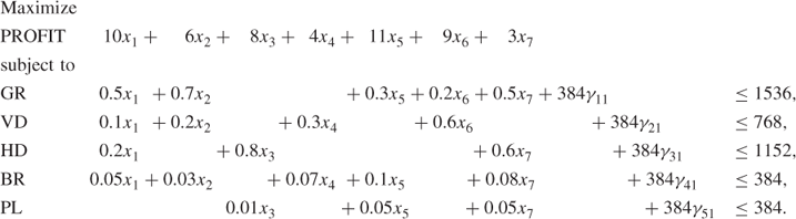
The upper market bounds would still apply together with upper bounds on the new integer variables.

The extension to a multi-period model would be similar to that described from the original problem.

It is necessary to ensure that each machine (apart from the grinders) is down for maintenance once in six months. This is achieved by the following constraints:

The new model therefore has five extra constraints.

Clearly, the solution to the original problem implies a feasible (though probably non-optimal) solution to the new problem. The optimal objective value obtained there can usefully be used as a cut-off value in the tree search.

An alternative formulation is possible using a 0–1 variable to indicate for each machine whether it is down for maintenance in a particular month or not. Such a formulation would have more variables and suffer the drawback, mentioned in Section 10.1, of producing equivalent alternate solutions in the tree search.

13.5 Manpower planning

A number of applications of linear programming to manpower planning have been published. Selected references are Davies (1973), Price and Piskor (1972), who apply goal programming, and Vajda (1975).

In order to formulate the problem presented here, it will be assumed that everything happens on the first day of each year. Clearly, this assumption is far from the truth. It is necessary to make some such assumption as it is only possible to represent quantities at discrete points of time if linear programming is to be applied.

On the first day of each year the following changes will take place simultaneously:

13.5.1 Variables

Strength of Labour Force

t_SKi = number of skilled workers employed in year i

t_SSi = number of semi-skilled workers employed in year i

t_USi = number of unskilled workers employed in year i

Recruitment

u_SKi = number of skilled workers recruited in year i

u_SSi = number of semi-skilled workers recruited in year i

u_USi = number of unskilled workers recruited in year i

Retraining

v_USSSi = number of unskilled workers retrained to semi-skilled in year i

v_SSSKi = number of semi-skilled workers retrained to skilled in year i

Downgrading

v_SKSSi = number of skilled workers downgraded to semi-skilled in year i

u_SKUSi = number of skilled workers downgraded to unskilled in year i

v_SSUSi = number of semi-skilled workers downgraded to unskilled in year i

Redundancy

w_SKi = number of skilled workers made redundant in year i

w_SSi = number of semi-skilled workers made redundant in year i

w_USi = number of unskilled workers made redundant in year i

Short-time Working

x_SKi = number of skilled workers on short-time working in year i

x_SSi = number of semi-skilled workers on short-time working in year i

x_USi = number of unskilled workers on short-time working in year i

Overmanning

y_SKi = number of superfluous skilled workers employed in year i

y_SSi = number of superfluous semi-skilled workers employed in year i

y_USi = number of superfluous unskilled workers employed in year i

13.5.2 Constraints

Continuity

Retraining Semi-skilled Workers

Overmanning

Requirements

13.5.3 Initial conditions

The initial conditions are t_SK0 = 1000, t_SS0 = 1500, t_US0 = 2000.

Some variables have upper bounds. These are (for i = 1, 2, 3)

Recruitment	Short-time working	Retraining
uSKi ≤ 500	xSKi ≤ 50	vUSSSi ≤ 200
uSSi ≤ 800	xSSi ≤ 50
uUSi ≤ 500	xUSi ≤ 50

To minimize redundancy, the objective function is

To minimize cost, the objective function is

This formulation has 24 constraints and 60 variables as well as simple upper bounds on 21 variables.

With most packages, it is convenient to incorporate both objectives into the model as ‘non-constraint’ rows. It is then possible to optimize both objectives within one computer run by means of the control program. In some packages, it is possible to form a composite objective through the control program, taking a certain linear combination of the original objectives. Alternatively, one of the objectives can be made a constraint. For a model such as this, with only two objectives, the most efficient way of investigating their effect is to treat one as a constraint and to perform parametric programming on its right-hand side.

13.6 Refinery optimization

The petroleum industry is the major user of linear programming models. This is a very small version of a typical application. Generally, the models used will consist of thousands of constraints, linking together possibly more than one oil refinery, giving a structured model as described in Section 4.1. The application of linear programming in the petroleum industry is described by Manne (1956).

13.6.1 Variables

In view of the many different sorts of variables in a model of this sort, it is convenient to use mnemonic names in this description of the formulation. The following variables are used to represent quantities of the materials (measured in barrels):

CRA	crude 1
CRB	crude 2
LN	light naphtha
MN	medium naphtha
HN	heavy naphtha
LO	light oil
HO	heavy oil
R	residuum
LNRG	light naphtha used to produce reformed gasoline
MNRG	medium naphtha used to produce reformed gasoline
HNRG	heavy naphtha used to produce reformed gasoline
RG	reformed gasoline
LOCGO	light oil used to produce cracked oil and cracked gasoline
HOCGO	heavy oil used to produce cracked oil and cracked gasoline
CG	cracked gasoline
CO	cracked oil
LNPMF	light naphtha used to produce premium motor fuel
LNRMF	light naphtha used to produce regular motor fuel
MNPMF	medium naphtha used to produce premium motor fuel
MNRMF	medium naphtha used to produce regular motor fuel
HNPMF	heavy naphtha used to produce premium motor fuel
HNRMF	heavy naphtha used to produce regular motor fuel
RGPMF	reformed gasoline used to produce premium motor fuel
RGRMF	reformed gasoline used to produce regular motor fuel
CGPMF	cracked gasoline used to produce premium motor fuel
CGRMF	cracked gasoline used to produce regular motor fuel
LOJF	light oil used to produce jet fuel
HOJF	heavy oil used to produce jet fuel
RJF	residuum used to produce jet fuel
COJF	cracked oil used to produce jet fuel
RLBO	residuum used to produce lube-oil
PMF	premium motor fuel
RMF	regular motor fuel
JF	jet fuel
FO	fuel oil
LBO	lube-oil

There are 36 such variables.

13.6.2 Constraints

Availabilities

The limited availability of the crude oils gives simple upper bounding constraints:

Capacities

The distillation capacity constraint is

The reforming capacity constraint is

The cracking capacity constraint is

The stipulation concerning production of lube-oil gives the following lowerand upper bounding constraints:

Continuities

The quantity of light naphtha produced depends on the quantities of the crudeoil used, taking into account the way in which each crude splits underdistillation. This gives

Similar constraints exist for MN, HN, LO, HO and R.

The quantity of reformed gasoline produced depends on the quantities of thenaphthas used in the reforming process. This gives the constraint

The quantities of cracked oil and cracked gasoline produced depend on thequantities of light and heavy oil used. This gives the constraints

The quantity of lube-oil produced (and sold) is 0.5 times the quantity ofresiduum used. This gives

The quantities of light naphtha used for reforming and blending are equal tothe quantities available. This gives

Similar constraints exist for MN and HN.

The quantities of light oil used for cracking and blending are equal to thequantities available.

For the blending of fuel oil, the proportion of light oil is fixed at 10/18.Therefore separate variables have not been introduced for this proportion asit is determined by the variable LO. This gives

Similar constraints exist for HO, CO and R, also involving fixed proportionsof FO, and for CG and RG.

The quantity of premium motor fuel produced is equal to the total quantity ofits ingredients. This gives

Similar constraints exist for RMF and JF.

Premium motor fuel production must be at least 40% of regular motor fuelproduction, giving

Qualities

It is necessary to stipulate that the octane number of premium motor fuel doesnot drop below 94. This is done by the constraint

There is a similar constraint for RMF.

For jet fuel we have the constraint imposed by vapour pressure. This is

This model has 29 constraints together with simple bounds on threevariables.

Some comment should be made concerning the blending of fuel oil where the ingredients (light, heavy, and cracked oil and residuum) are taken in fixed proportions. Here it might be preferable to think of the production of FO as an activity. It is common in the oil industry to think in terms of activities rather than quantities. In Section 3.4, modal formulations are discussed where activities represent the extreme modes of operation of a process. Here we have a special case of a process with one mode of operation. The level of this activity then fixes the proportions of the ingredients, in a case such as this, automatically.

13.6.3 Objective

The only variables involving a profit (or cost) are the final products. This gives an objective (in pounds) to be maximized of

13.7 Mining

This problem has a combinatorial character. In each year a choice of up to three out of the four possible mines must be chosen for working. There are 15 ways of doing this each year, giving a total of 15⁵ possible ways of working over five years. For larger problems with, say, 15 mines being considered over 20 years the number of possibilities will be astronomical. By using integer programming, with the branch and bound method, only a fraction of these possibilities need be investigated.

0–1 variables are introduced to represent decisions whether to work or not to work a particular mine in a certain year. The different sorts of variables are described below.

13.7.1 Variables

There are 20 such 0–1 integer variables.

There are 20 such 0–1 integer variables.

There are 20 such continuous variables.

There are five such continuous variables.

In total, there are therefore 65 variables, of which 40 are integer.

13.7.2 Constraints

M_i is the maximum yearly output from mine i. This constraint implies that if mine i is not worked in year t there can be no output from it in that year. There are 20 such constraints.

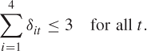
This constraint allows no more than three mines to be worked in any year. There are five such constraints.

According to this constraint, if mine i is ‘closed’ in year t_, it cannot be worked in that year. There are 20 such constraints.

This forces a mine to be closed in all years subsequent to that in which it is first closed. There are 16 such constraints.

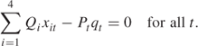
Q_i is the quality of the ore from mine i and P_t the quality required in year t. There are five such blending constraints.

This constraint ensures that the tonnage of blended ore in each year equals the combined tonnage of the constituents. There are five such constraints.

In total there are 71 constraints.

13.7.3 Objective

The total profit consists of the income from selling the blended ore minus the royalties payable. This is to be maximized. It can be written

R_it is the royalty payable on mine i in year t discounted at a rate of 10% per annum. I_t is the selling price of each ton of blended ore in year t discounted at a rate of 10% per annum. The advantage of this formulation of the problem over an alternative one is discussed by Williams (1978).

There would seem to be advantage in this model in working mines early in the hope that they may be closed permanently later. In addition, the discounting of revenue gives an advantage to working mines early. The suggested solution strategy is therefore to branch on the variables δ_it, giving priority to low values of t.

13.8 Farm planning

This problem is based on that of Swart et al. (1975). By only considering five years, the model can be kept reasonably small but inevitably much of the realism is lost.

There are a number of different ways of formulating this problem. In the formulation suggested here, a large number of variables are introduced whose values are effectively fixed by the constraints of the model. These variables represent the numbers of cows of different ages in each year. For example, the number of cows of ages 1, 2, and so on, in year 1 will be determined by the initial numbers of cows given in year 0. Similarly, the numbers of cows of ages 2, 3 and so on, in year 2 will be fixed. It would therefore be possible to calculate the values of all these variables and not introduce them into the model. While this would make for a more compact model, it would not be as easy to understand. Nor does it seem worthwhile to carry out manual calculation best done by a computer. The most satisfactory course of action is to reduce or presolve the model in order to determine the fixed values of these variables. Experience with doing this is reported with the solution in Part IV.

13.8.1 Variables

x_it = number of tons of grain grown on group i land in year t

y_t = number of tons of sugar beet grown in year t

z_t = number of tons of grain bought in year t

s_t = number of tons of grain sold in year t

u_t = number of tons of sugar beet bought in year t

v_t = number of tons of sugar beet sold in year t

l_t = extra labour recruited in year t (in units of 100 hours)

m_t = capital outlay in year t (in units of £200)

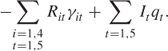
n_t = number of heifers sold at birth in year t

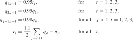
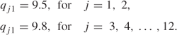
q_jt = number of cows of age j years in year t

r_t = number of cows of age 0 in year t

p_t = profit in year t

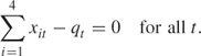
i = 1, 2, 3, 4; t = 1, 2, 3, 4, 5 and j = 1, 2, …, 12. (A variable n₆ is also defined to allow heifers to be sold at the beginning of the sixth year.)

As with other planning models, it is necessary to consider discrete intervals of time and assume changes occur once in each interval. In this case, we assume changes occur once each year.

13.8.2 Constraints

Continuity

Initial Conditions (Fixed Variables)

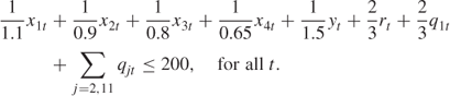
Accommodation

Grain Consumption

Sugar Beet Consumption

Grain Growing

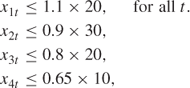
Acreage

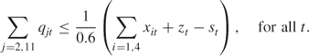
Labour (in 100 hours)

End Total

(This constraint may be specified by a range of 125 on the previous constraint.)

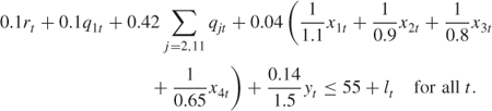
Profit

(The annual repayment on a £200 loan is £39.71.)

Profit Can Never be Negative

(The main effect of this constraint is to limit capital expenditure to cash available.)

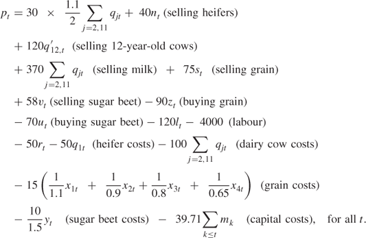
13.8.3 Objective function

In order to make capital expenditure as ‘costly’ in latter years as in former ones, it is necessary to take account of repayments beyond the five years. This gives an objective function (to be maximized):

The costs incurred by the repayments beyond the five years must be credited back when the final profit over the five years is obtained.

This model has 84 constraints and 130 variables.

13.9 Economic planning

The model resulting from this problem is a dynamic Leontief model of the type mentioned in Section 5.2. A rather similar model has been considered by Wagner (1957).

13.9.1 Variables

x_it = total output of industry i in year t(i = C (coal), S(steel), T(transport), t = 1, 2, …, 5)

s_it = stock level of industry i at the beginning of year t

y_it = extra productive capacity for industry i becoming effective in year t(t = 2, 3, …, 6)

13.9.2 Constraints

Total Input

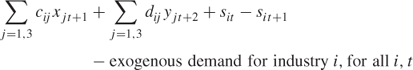
( are initial stocks given), where c_ij and d_ij are the input/output coefficients in the first three rows of Tables 12.1 and 12.2 respectively in the statement of the problem.

Manpower

Productive Capacity

In order to build a realistic model, it is necessary to think beyond the end of the five-year period. To ignore exogenous demand in the sixth and subsequent years would result in no inputs being accounted for in the fifth year. We therefore assume that exogenous demand remains constant up to and beyond year 5, the stock level remains constant, and that there is no increase in productive capacity after year 5. In order to find the inputs to each industry in year 5, we simply have to solve a static Leontief model:

x_i is the (static) output from industry i in year 5 and beyond.

This set of three equations gives lower limits to the variables, giving

In the total output constraint above, x_it will be set greater than or equal to these values for t ≥ 6. y_it will be set to 0 for t ≥ 6.

13.9.3 Objective function

This model has 45 variables and 42 constraints.

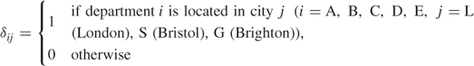
13.10 Decentralization

This is a modified form of the quadratic assignment problem described in Section 9.5. Methods of solving such problems are described by Lawler (1974). The problem presented here is based on the problem described by Beale and Tomlin (1972). They treat their problem by linearizing the quadratic terms and reducing the problem to a 0–1 integer programming problem. We adopt the same approach here.

13.10.1 Variables

There are 15 such 0–1 variables.

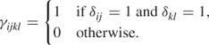
γ_ijkl is only defined for i < k and C_ik ≠ 0. There are 54 such 0–1 variables.

13.10.2 Constraints

Each department must be located in exactly one city. This gives the constraints

There are five such constraints. These constraints can be treated as special ordered sets of type 1 as described in Section 9.3.

No city may be the location for more than three departments. This gives the constraints

There are three such constraints.

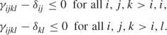
Using the variables δ_ij together with the two types of constraint above, we could formulate a model with an objective function involving some quadratic terms δ_ijδ_kl. Instead, these terms are replaced by the 0–1 variables γ_ijkl giving a linear objective function. It is, however, necessary to relate these new variables to the δ_ij variables correctly. To do this we model the relations

and

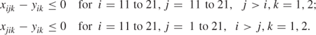
Following the discussion in Section 9.2, the first conditions can be achieved by the following constraints:

There are 108 such constraints.

The second conditions are achieved by the constraints

There are 54 such constraints.

13.10.3 Objective

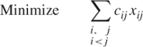
The objective is to minimize

where B_ij is the benefit to be gained from locating department i in city j as given in Part II (for j = L (London), B_ij = 0). C_ik and D_ji are given in the tables in Part II, Section 12.10.

This model has 162 constraints and 69 variables (all 0–1).

Beale and Tomlin formulate their model more compactly. As a consequence, the corresponding linear programming problem is much less constrained than it might be (see Section 10.1). They then expand some of the constraints. Use is then made of the branching strategy to avoid expanding other constraints.

13.11 Curve fitting

This is an application of the goal programming type of formulation discussed in Section 3.3. Each pair of corresponding data values (x_i, y_i) gives rise to a constraint. For cases (1) and (2), these constraints are

x_i and y_i are constants (the given values); b, a, u_i and v_i are variables. u_i and v_i give the amounts by which the values of y_i proposed by the linear expression differ from the observed values. It is important to allow a and b to be ‘free’ variables, that is, they can be allowed to take negative as well as positive values.

In case (1) the objective is to minimize

This model has 19 constraints and 40 variables.

In case (2) it is necessary to introduce another variable z together with 38 more constraints:

The objective, in this case, is simply to minimize z. This minimum value of z will clearly be exactly equal to the maximum value of v_i and u_i.

In case (3), it is necessary to introduce a new (free) variable c into the first set of constraints to give

The same objective functions as in (1) and (2) will apply.

It is much more usual in statistical problems to minimize the sum of squares of the deviations as the resultant curve often has desirable statistical properties. There are, however, some circumstances in which a sum of absolute deviations is acceptable or even more desirable. Moreover, the possibility of solving this type of problem by linear programming makes it computationally easy to deal with large quantities of data.

Minimizing the maximum deviation has certain attractions from the point of view of presentation. The possibility of a single data point appearing a long way off the fitted curve is minimized.

13.12 Logical design

In order to simplify the formulation, the optimal circuit can be assumed to be a subnet of the maximum shown in Figure 13.1. The following 0–1 integer variables are used:

x_ij is the output from gate i for the combination of external input signals specified in the jth row of the truth table.

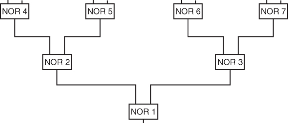
The following constraints are imposed.

A NOR gate can only have an external input if it exists. These conditions are imposed by the constraints

If a NOR gate has one (or two) external inputs leading into it, only one (or no) NOR gates can feed into it. These conditions are imposed by the constraints

where j and k are the two NOR gates leading into i in Figure 13.1.

The output signal from NOR gate i must be the correct logical function (NOR) of the input signals into gate i if gate i exists. Let α_1j (a constant) be the value of the external input signal A in the jth row of the truth table. Similarly α_2j corresponds to the external input signal B. These conditions give

The above six classes of constraints are defined for l = 1, 2, …, 4, where j and k are the NOR gates leading into gate i in Figure 13.1. As the α_ij are constants, some of the above constraints are redundant for particular values of l and may be ignored.

For NOR gate 1, the x_1l variables are fixed at the values specified in the truth table, that is,

If there is an output signal of 1 from a particular NOR gate for any combination of the input signals, then that gate must exist.

In order to avoid a trivial solution containing no NOR gates, it is necessary to impose a constraint such as

The objective is to minimize ∑_is_i.

This model has 154 constraints and 49 variables (all 0–1), including the four fixed variables. The redundant constraints are included in this total.

13.13 Market sharing

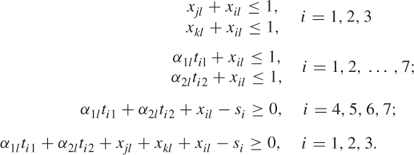
This problem can be formulated as an integer programming model where each of the 23 retailers is represented by a 0–1 variable δ_i. If δ_i = 1 retailer i is assigned to division D1. Otherwise, the retailer is assigned to division D2. Slack and surplus variables can be introduced into each constraint to provide the required objective, which is to minimize the sum of the proportionate deviations from the desired ‘goals’ of the 40/60 splits. For example, in the oil market in region 3, we have a total market of 100 (10⁶ gallons). In order to split this 40/60, we have the constraint

y₁ and y₂ are slack and surplus variables which are given a cost of 0.01 in the first objective function. y₁ and y₂ are also given simple upper bounds of 5. The other ‘goal’ constraints can be treated in a similar fashion.

In order to define the second ‘minimax’ objective, we need to introduce a variable z together with the constraints

for all slack and surplus variables y_i, where w_i is the total quantity for the 40% goal constraint with which y_i is associated. The second objective is then simply to minimize z.

The resultant model has 18 constraints and 36 variables, of which 23 are 0–1.

As it stands, this model is a correct representation of the problem but could prove difficult to solve as one feasible integer solution need bear no resemblance to another one. In consequence, the tree search for the optimal integer solution could be fairly random. As the results in Section 14.13 suggest, this model did prove difficult to solve optimally. One approach to reformulating the problem is to replace some of the constraints by ‘facet’ constraints in the manner described in Section 10.2. For example, the goal constraint above is equivalent to

The first of these constraints can be augmented by the following constraints obtained from strong covers:

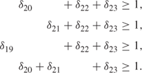
The second of the constraints can be augmented by the constraints

All the other constraints could be treated in a similar fashion. Unfortunately, the number of such ‘facet’ constraints derivable from each of the goal constraints for (1) and (2) in the statement of the problem in Section 12.13 proved prohibitively large. There are, however, a large but manageable number which can be derived from (3) and (4) together with those above for (5). In total, the number of such constraints turned out to be 228. They were enumerated in a trivial amount of time, using the method described in Section 10.2.

It is still necessary to retain the original constraints, with their slack and surplus variables providing an objective function, as we are only adding in some of the ‘facet’ constraints for each goal constraint.

Unfortunately, this augmented formulation proved difficult to solve largely as a result of its increased size.

A third possibility is to replace some of the goal constraints by single tighter constraints. How this may be done for a general 0–1 constraint is described by Bradley et al. (1974). An example of such a single constraint simplification is provided by the problem OPTIMIZING A CONSTRAINT, in Section 13.18.

The three goal constraints for (3)–(5) in Section 12.6.1 can be written as three pairs of constraints:

Using the method referenced above, it is possible to give six constraints that have equivalent sets of 0–1 solutions but are ‘tighter’ in a linear programming sense. These are

Each of these constraints is the equivalent one, to the corresponding one above, which has the smallest right-hand side coefficient. These tighter constraints were derived in a trivial amount of time using linear programming. Details of the method are described with the example, OPTIMIZING A CONSTRAINT, in Section 13.18.

It is still necessary to retain the original constraints with their slack and surplus variables needed in the objective function. This reformulation proved the most successful. Computational experience is given with the solution in Section 14.13.

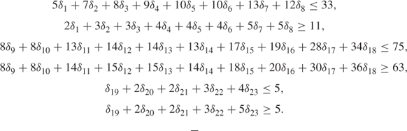
13.14 Opencast mining

This problem can be formulated as a pure 0–1 programming problem by introducing 0–1 variables δ_i and numbering the blocks:

If a block is extracted, then the four blocks above it must also be extracted. Suppose, for example, that the numbering were such that blocks 2– 5 were directly above 1. The condition could then be imposed by the four constraints

Similar constraints can be imposed for all other blocks (apart from those on the surface).

The objective is to maximize

where

This formulation has the extremely important property described in Section 10.1. Each constraint contains one coefficient +1 and one coefficient −1. This guarantees a totally unimodular matrix. If the model is solved as a continuous linear programming model, the optimal solution will be integer automatically. There is therefore no need to use, computationally much more costly, integer programming.

This property makes it possible to solve much larger versions of this problem in a reasonable amount of time. As described in Section 10.1, the dual of this linear programming model is a network flow problem and could be solved very efficiently by a specialized network flow algorithm, see Williams (1982).

The model has 56 constraints and 30 variables. Each variable has an upper bound of 1.

13.15 Tariff rates (power generation)

This problem is based on a model described by Garver (1963). The following formulation is suggested here.

13.15.1 Variables

n_ij = number of generating units of type i working in period j (where j = 1, 2, 3, 4, and 5 are the five periods of the day listed in the question)

s_ij = number of generators of type i started up in period j

x_ij = total output rate from generators of type i in period j

x_ij are continuous variables; n_ij and s_ij are general integer variables.

13.15.2 Constraints

Demand must be met in each period:

where D_j is demand given in period j.

Output must lie within the limits of the generators working:

where m_i and M_i are the given minimum and maximum output levels for generators of type i.

The extra guaranteed load requirement must be able to be met without starting up any more generators:

The number of generators started in period j must equal the increase in number:

where n_ij is number of generators started in period j (when j = 1, period j–1 is taken as 5).

In addition, all the integer variables have simple upper bounds corresponding to the total number of generators of each type.

13.15.3 Objective function (to be minimized)

where C_ij are costs per hour per megawatt above minimum level multiplied by the number of hours in the period; E_ij are costs per hour for operating at minimum level multiplied by the number of hours in the period and F_i are start-up costs.

This model has a total of 55 constraints and 30 simple upper bounds. There are 45 variables, of which 30 are general integer variables.

13.16 Hydro power

The model described in Section 13.15 can be extended by additional variables and constraints.

13.16.1 Variables

h_ij = 1 if hydro of type i working in period j

= 0 otherwise

where i = 1, 2

t_ij = 1 if hydro of type i started in period j

= 0 otherwise

l_j = height of reservoir at beginning of period j

p_j = number of megawatts of pumping in period j

13.16.2 Constraints

The demand constraint becomes

where L_i is the operating level of hydro i.

Reservoir level changes resulting from pumping and generation give

where T_j is number of hours in period j and R_i is height reduction per hour caused by hydro j.

The extra load guarantee requirement becomes

The number of hydros started in period j must equal the increase in number:

13.16.3 Objective function (to be minimized)

This needs to be augmented by the terms

where K_i is the cost per hour of hydro i and G_i is the start-up cost of hydro i.

This model has 55 constraints, 25 upper bounds and 75 variables, of which 50 are integer.

13.17 Three-dimensional noughts and crosses

This ‘pure’ problem is included as it typifies the combinatorial character of quite a lot of integer programming problems. Clearly, there are an enormous number of ways of arranging the balls in the three-dimensional array. Such problems often prove difficult to solve as integer programming models. There is advantage to be gained from using a heuristic solution first. This solution can then be used to obtain a cut-off value for the branch and bound tree search as described in Section 8.3. A discussion of two possible ways of formulating this problem is given in Williams (1974). The better of those formulations is described here.

13.17.1 Variables

The cells are numbered from 1 to 27. It is convenient to number sequentially row by row and section by section. Associated with each cell a 0–1 variable δ_j is introduced with the following interpretation:

There are 27 such 0–1 variables.

There are 49 possible lines in the cube. With each of these lines, we associate a 0–1 variable γ_i with the following interpretations:

There are 49 such 0–1 variables.

13.17.2 Constraints

We wish to ensure that the values of the variables γ_i truly represent the conditions above. In order to do this, we have to model the condition

where i1, i2, and i3 are the numbers of the cells in line i.

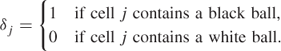
This condition can be modelled by the constraints

In fact, these constraints do not ensure that if γ_i = 1 all balls will be of the same colour in the line. When the objective is formulated, it will be clear that this condition will be guaranteed by optimality.

In order to limit the black balls to 14, we impose the constraint

There are a total of 99 constraints.

13.17.3 Objective

In order to minimize the number of lines with balls of a similar colour, we minimize

In total, this model has 99 constraints and 76 0–1 variables.

13.18 Optimizing a constraint

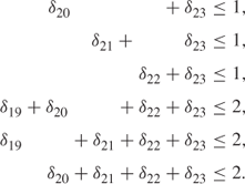
A procedure for simplifying a single 0–1 constraint has been described by Bradley et al. (1974). We adopt their procedure of using a linear programming model. It is convenient to consider the constraint in a standard form with positive coefficients in descending order of magnitude. This can be achieved by the transformation

giving

We wish to find another equivalent constraint of the form

The a_i coefficients become variables in the linear programming model. In order to capture the total logical import of the original constraint, we search for subsets of the indices known as roofs and ceilings. Ceilings are ‘maximal’ subsets of the indices of the variables for which the sum of the corresponding coefficients does not exceed the right-hand side coefficient. Such a subset is maximal in the sense that no subset properly containing it, or to the left in the implied lexicographical ordering, can also be a ceiling. For example, the subset {1, 2, 4, 8} is a ceiling, 23 + 21 + 17 + 9 ≤ 70, but any subset properly containing it (e.g. {1, 2, 4, 7, 8}) or to the ‘left’ of it (e.g. {1, 2, 4, 7}) is not a ceiling. Roofs are ‘minimal’ subsets of the indices for which the sum of the corresponding coefficients exceeds the right-hand side coefficient. Such a subset is ‘minimal’ in the same sense as a subset is ‘maximal’. For example {2, 3, 4, 5} is a roof, 21 + 19 + 17 + 14 > 70, but any subset properly contained in it (e.g. {3, 4, 5}) or to the ‘right’ of it (e.g. {2, 3, 4, 6}) is not a roof.

If {i₁, i₂, …, i_r} is a ceiling, the following condition among the new coefficients a_i is implied:

If {i₁, i₂, …, i_r} is a roof, the following condition among the new coefficients a_i is implied:

It is also necessary to guarantee the ordering of the coefficients. This can be done by the series of constraints

If these constraints are given together with each constraint corresponding to a roof or ceiling, then this is a sufficient set of conditions to guarantee that the new 0–1 constraint has exactly the same set of feasible 0–1 solutions as the original 0–1 constraint.

In order to pursue the first objective, we minimize a₀−a₃−a₅ subject to these constraints.

For the second objective, we minimize

For this example, the set of ceilings is

The set of roofs is

The resultant model has 19 constraints and 9 variables.

If the constraint were to involve general integer rather than 0–1 variables, then we could still formulate the simplification problem in a similar manner after first converting the constraint to one involving 0–1 variables in the way described in Section 10.1. It is, however, necessary to ensure, by extra constraints in our LP model, the correct relationship between the coefficients in the simplified 0–1 form. How this may be done is described in Section 10.2.

13.19 Distribution 1

This problem can be regarded as one of finding the minimum cost flow through a network. Such network flow problems have been extensively treated in the mathematical programming literature. A standard reference is Ford and Fulkerson (1962). Specialized algorithms exist for solving such problems and are described in Ford and Fulkerson (1962), Jensen and Barnes (1980), Glover and Klingman (1977) and Bradley (1975).

It is, however, always possible to formulate such problems as ordinary linear programming models. Such models have the total unimodularity property described in Section 10.1. This property guarantees that the optimal solution to the LP problem will be integer as long as the right-hand side coefficients are integer.

We choose to formulate this problem as an ordinary LP model in order that we may use the standard revised simplex algorithm. There would be virtue in using a specialized algorithm. The special features of this sort of problem, which also make the use of a specialized algorithm worthwhile, fortunately, make the problem fairly easy to solve as an ordinary LP problem. Sometimes, however, when formulated in this way, the resultant model is very large. The use of a specialized algorithm then also becomes desirable as it results in a compact representation of the problem. As the example presented is very small, such considerations do not arise here.

The factories, depots and customers will be numbered as below:

Factories	1	Liverpool
	2	Brighton
Depots	1	Newcastle
	2	Birmingham
	3	London
	4	Exeter
Customers	C1, C2,…, C6

13.19.1 Variables

x_ij = quantity sent from factory i to depot j, i = 1, 2, j = 1, 2, 3, 4

y_ik = quantity sent from factory i to customer k, i = 1, 2, k = 1, 2, …, 6

z_jk = quantity sent from depot j to customer k, j = 1, 2, 3, 4, k = 1, 2, …, 6

There are 44 such variables.

13.19.2 Constraints

Factory Capacities

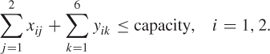
Quantity into Depots

Quantity out of Depots

Customer Requirements

The capacity, quantity and requirement figures are given with the statement of the problem in Part II.

There are 16 such constraints.

13.19.3 Objectives

The first objective is to minimize cost. This is given by

where the coefficients c_ij, d_ik and e_jk are given with the problem in Part II.

The second objective will take the same form as that above, but this time, the c_ij, d_ik and e_jk will be defined as below:

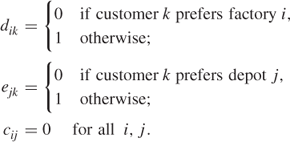
This objective is to be minimized.

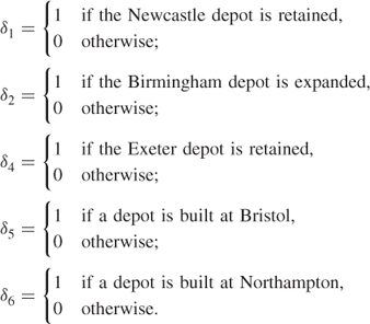
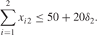
13.20 Depot location (distribution 2)

The linear programming formulation of the distribution problem can be extended to a mixed integer model to deal with the extra decisions of whether to build or close down depots. Extra 0–1 integer variables are introduced with the following interpretations:

In addition, extra continuous variables , , z_5k and z_6k are introduced to represent quantities sent to and from the new depots.

The following constraints are added to the model.

If a depot is closed down or not built, then nothing can be supplied to it or from it:

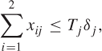
where T_j is the capacity of depot j.

From Birmingham the quantity supplied to and from the depot must lie within the extension:

There can be no more than four depots (including Birmingham and London):

In the objective function, the new x_ij and z_jk variables are given their appropriate costs. The additional expression involving the δ_j variables is added to the objective function:

This model has 21 constraints and 65 variables (five are integer and 0–1).

13.21 Agricultural pricing

This problem is based on that described by Louwes et al. (1963).

Let x_M, x_B, x_C1 and x_C2 be the quantities of milk, butter, cheese 1 and cheese 2 consumed (in thousands of tons) and p_M, p_B, p_C1 and p_C2 their respective prices (in £1000 per ton).

The limited availabilities of fat and dry matter give the following two constraints:

The price index limitation gives (measured in £1000)

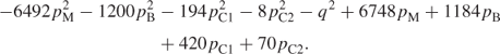
The objective is to maximize ∑_ix_ip_i.

In addition the x variables are related to the p variables through the price elasticity relationships:

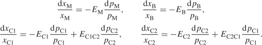
These differential equations can easily be integrated to give the x variables as expressions involving the p variables. If these expressions are substituted in the above constraints and the objective function, non-linearities are introduced into the first two constraints as well as the objective function. The non-linearities could be separated and approximated to by piecewise linear functions as described in Section 7.4.

In order to reduce the number of non-linearities in the model, the relationships implied by the differential equations above can be approximated to by the linear relationships:

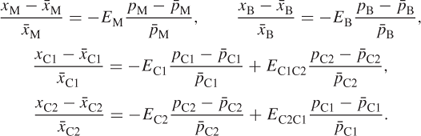
and are the known quantities consumed with their prices for the previous year. The approximation can be regarded as warranted if the resultant values of x and p do not differ significantly from and .

Using the above relationships to substitute for the x variables in the first two constraints and the objective function gives the model

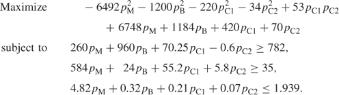
In addition, it is necessary to represent explicitly the non-negativity conditions on the x variables. These give

This is a quadratic programming model as there are quadratic terms in the objective function. Special algorithms exist for obtaining a, possibly, local optimum such as that of Beale (1959). In order to solve the model with a standard package (if this does not have a quadratic programming facility), we can convert it into a separable form and approximate the non-linear terms by piecewise linear expressions.

In order to put this model into a separable form, it is necessary to remove the term p_C1p_C2. This may be done by introducing a new variable q together with the constraint

(It is important to allow q to be negative, if necessary, by incorporating it in the model as a ‘free’ variable.)

The objective function can then be written in the separable form (a sum of non-linear functions of single variables):

This transformation also demonstrates that the model is convex (as described in Section 7.2). Using a piecewise linear approximation to the non-linearities, there is therefore no danger of obtaining a local optimum with separable programming. In fact, it is sufficient to use the conventional simplex algorithm. This will enable one to obtain a true (global) optimum.

Nevertheless, there is no guarantee that models of this sort (if the price elasticities had been different) will always be convex. Then it would be necessary to use integer programming to guarantee a global optimum or separable programming to produce a local optimum.

The solution given in Part IV is based on grids where p_i, q and and q² are defined in intervals of width 0.05. It is only necessary to define the grids within the possible ranges of values which p_i and q can take. These ranges can be found by examining the constraints of the model or by using linear programming to successively maximize and minimize the individual variables p_i and q subject to the constraints.

13.22 Efficiency analysis

There are a number of linear programming formulations of the DEA problem. Fuller coverage of the subject can be found in Farrell (1957), Charnes et al. (1978) and Thanassoulis et al. (1987). The formulation we give here is well described in Land (1991). It should be pointed out that there is also a dual formulation that is commonly used and relies on finding weighted ratios of outputs to inputs using the technique mentioned in Section 3.2. This formulation can be found in the above references.

For garage j suppose its six inputs are a_1j to a_6j and its three outputs are a_7j to a_9j. If we choose a specific garage k, we will seek to find a mixture of the 28 garages whose combined inputs do not exceed those of k but whose combined output does. Let us choose x_j units of each of the garages. Our constraints are then

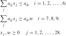
If we choose to maximize w then, so long as we can make w larger than 1, we will have chosen a mixture of garages whose combined inputs do not exceed that of the garage under consideration but whose combined outputs do exceed some of the outputs, demonstrating its inefficiency compared with this mixture. 1/w is usually referred to as the efficiency number.

Should it not be possible to find such a mixture, then the result will be to use one unit of the garage itself, resulting in a value of 1 for w.

In order to solve this problem, it is necessary to solve the model 28 times for each value of k. With some modelling/optimization systems, it is possible to do this automatically.

13.23 Milk collection

This problem is an extension of the travelling salesman problem whose formulation is discussed in Section 9.5. We extend the formulation given there.

13.23.1 Variables

13.23.2 Constraints

The limited tanker capacity gives

where K_i is the daily pickup requirement from farm i and C is the tanker capacity.

The limit on visiting some farms only every other day gives

The need to visit the ‘every day’ farms on each tour gives

The need to visit the ‘every other day’ farms on the chosen day gives

Taking into account the considerations discussed in Chapter 10, these constraints imply those below for which the associated linear programming relaxation is more constrained, making the model much easier to solve:

In order to prevent unnecessary (and computationally more costly) symmetric alternative solutions (switching days of visiting farms), it is convenient to set y_11,1 to 1, forcing farm 11 to be visited on the first day.

13.23.3 Objective

where c_ij is the distance between farm i and farm j.

This model has 65 constraints and 442 variables (all 0–1 integer).

As it is only a relaxation of the true model (the subtour elimination constraints have been ignored), it will almost certainly be necessary to add these on an ‘as needed’ basis during the course of optimization in a similar manner as for the travelling salesman problem, as described in Section 9.5.

13.24 Yield management

In order to solve this problem, a stochastic program (as mentioned in Section 1.2) will be built. This will be a three-period model. Solving the model for the first time will give recommended price levels and sales three weeks from departure and recommended price levels and sales for subsequent weeks under all possible scenarios. Account will be taken of the probabilities of these scenarios in order to maximize expected yield. A week later the model will be rerun, taking into account the committed sales and revenue in the first week, to redetermine recommended prices and sales for the second week (i.e. with ‘recourse’) and the third week under all possible scenarios. The procedure will be repeated again a week later.

13.24.1 Variables

p_1ch = 1 if price option h chosen for class c in week 1

= 0 otherwise (c = 1, 2, 3, h = 1, 2, 3)

p_2ich = 1 if price option h chosen for class c in week 2 as a result of scenario i in week 1

= 0 otherwise (c = 1, 2, 3, h = 1, 2, 3, i = 1, 2, 3)

p_3ijch = 1 if price option h chosen for class c in week 3 as a result of scenario i in week 1 and scenario j in week 2

= 0 otherwise

s_1ich = number of tickets sold in week 1 for class c under price option h and scenario i

s_2ijch = number of tickets sold in week 2 for class c under price option h if scenario i holds in week 1 and scenario j in week 2

s_3ijkch = number of tickets sold in week 3 for class c under price option if scenario i holds in week 1, scenario j in week 2 and scenario k in week 3

r_1ich = revenue in week 1 from class c under price option h and scenario i

r_2ijch = revenue in week 2 from class c under price option h if scenario i holds in week 1 and scenario j in week 2

r_3ijkch = revenue in week 3 from class c under price option h if scenario i holds in week 1, scenario j in week 2 and scenario k in week 3

u_ijkc = slack capacity in class c under scenarios i, j, k in successive weeks

v_ijkc = excess capacity in class c under scenarios i, j, k in successive weeks

n = number of planes to fly

While it is necessary to make the p variables 0–1 integer and n integer, the s variables can be treated as continuous and their values rounded.

13.24.2 Constraints

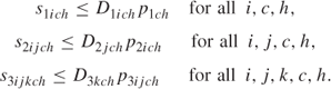
If a particular price option is chosen (under certain scenarios), then the sales cannot exceed the estimated demand and the revenue must be the product of the price and sales. These conditions can be imposed using the device described in Section 9.2 for modelling the product of a continuous and 0–1 integer variable.

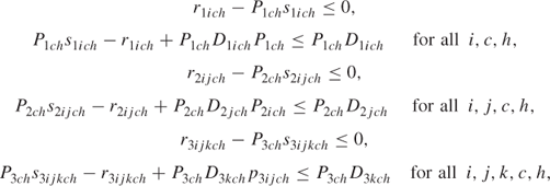
where P and D are the given prices and demands for the corresponding periods, scenarios, classes and options.

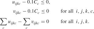
The seat capacities must be abided by for all scenarios:

where C_c is the given capacity per plane for class c.

Adjustment is possible between classes:

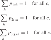
Exactly one price option must be chosen in each class under each set of scenarios:

The above set of constraints could be replaced by SOS1 sets without the need to declare the p variables integer.

Numbers sold cannot exceed demand:

Up to six planes can be flown:

13.24.3 Objective

(measuring in £1000) where Q_i is the probability of scenario i.

This model has 1200 constraints, one bound and 982 variables, of which 117 are 0–1 integer and one general integer.

In defining the data, it is desirable that the demands in the scenarios cover the extremes as well as the most likely cases. The recommended sales will not exceed those of the most extreme scenario in the solution to this model. In this example, it can be seen that final demands (known with hindsight) exceed those of all scenarios in a few cases. As a result, the solution will not result in sales to meet all of these demands.

Models for subsequent weeks (with recourse) are obtained from this model by fixing prices and sales for weeks that have elapsed.

13.25 Car rental 1

We model this problem as a deterministic linear programme. There would be advantage to be gained from modelling it as a stochastic programme. In order to do this, we would need to obtain data to quantify the uncertain demand.

13.25.1 Indices

i, j = Glasgow, Manchester, Birmingham, Plymouth

t = Monday, Tuesday, Wednesday, Thursday, Friday, Saturday

k = 1, 2, 3 (days hired)

Although this is a ‘dynamic’ problem, we seek a steady-state solution and can therefore regard the set of days as ‘circular’, that is, Monday of a week ‘follows’ after the subsequent Saturday; that is, if t = Monday then t − 1 = Saturday.

13.25.2 Given data

D_it = estimated rental demand at depot i on day t as given in Table 12.19

P_ij = proportion of cars rented at depot i to be returned to depot j as given in Table 12.21

C_ij = cost of transfer of a car from depot i to depot j as given in Table 12.22

Q_k = proportion of cars hired for k days

R_i = repair capacity of depot i

RCA_k = rental cost for k days with return to same depot as given in Table 12.23

RCB_k = rental cost for k days with return to another depot as given in Table 12.23

RCC = rental cost for Saturday with return to same depot on Monday

RCD = rental cost for Saturday with return to another depot on Monday

CS_k = marginal cost to company of k day hire of a car for all i, t

13.25.3 Variables

n = total number of cars owned

nu_it = number of undamaged cars at depot i at the beginning of day t for all i, t

nd_it = number of damaged cars at depot i at the beginning of day t for all i, t

tr_it = number of cars rented out from depot i at beginning of day t for all i, t

eu_it = undamaged cars left at depot i during day t for all i, t

ed_it = damaged cars left at depot i at the beginning of day t for all i, t

tu_ijt = number of undamaged cars at depot i at the beginning of day t, to be transferred to depot j for all i, j, t

td_ijt = number of damaged cars at depot i at the beginning of day t, transferred to depot t for all i, j, t

rp_it = number of damaged cars to be repaired at depot i on day for all i, t

13.25.4 Constraints

Total number of cars equals number hired out from all depots on Monday for 3 days, plus those on Tuesday for 2 or 3 days, plus all damaged and undamaged cars in depots at the beginning of Wednesday.

13.25.5 Objective

Note that £10 has been added to the profit on each rented car to reflect the surcharge of £100 charged on the 10% of cars that are returned damaged.

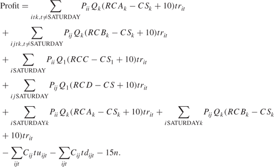
This model has a total of 84 constraints and 337 variables.

It is not necessary to constrain the w_ijkl to be non-negative. They can be regarded as ‘free’ variables. Avoiding these two stipulations helps the model to solve more easily.

13.26 Car rental 2

We introduce the following 0–1 integer variables with the following interpretations:

δ_B1 = 1, if the Birmingham repair capacity is expanded by 5 cars per day.

δ_B2 = 1, if the Birmingham repair capacity is expanded by a further 5 cars per day.

δ_M1 = 1, if the Manchester repair capacity is expanded by 5 cars per day.

δ_M2 = 1, if the Manchester repair capacity is expanded by a further 5 cars per day.

δ_P = 1, if the Plymouth repair capacity is expanded by 5 cars per day.

The following expression is added to the objective function:

together with the following extra constraints:

and the repair capacity constraints for Birmingham, Manchester and Plymouth have 5δ_B1 + 5δ_B2, 5δ_M1 + 5δ_M2 and 5δ_P, respectively added.

13.27 Lost baggage distribution

We formulate this problem as an integer programming model. It is an extension of the travelling salesman problem, discussed in section 9.5. It can be regarded as a (simple) case of the vehicle routing problem. In the problem here, there are no vehicle capacites and no time windows for the delivery to each location (apart from the overall 2 hours guarantee). Nevertheless, it is potentially a very difficult problem to solve, for more than a modest number of locations. Also it can give rise to a very large model. There are a number of different ways of formulating a model, which vary greatly in their size and difficuly of solution. We suggest a model that is practicable in both size and computational tractibility. Although the problem is ‘symmetric’ in the sense that the distance from X to Y is the same as that from Y to X, we extend the asymmetric formulation of the travelling salesman problem in order to give the ‘time’ to return to Heathrow, after a van has completed all its deliveries, as 0. In this way, only the total time taken to reach the last delivery is counted within the 2 hours time limit. We are therefore seeking a ‘Hamiltoniam path’ (as opposed to a circuit) for each van, starting from Heathrow.

13.27.1 Variables

All variables are 0–1 and integer

x_ijk = 1, iff van k visits, and goes directly from location i to j for all i, j, and k.

y_ik = 1, iff location i is visited by van k for all i, k.

δ_k = 1, iff van k is used.

13.27.2 Objective

Minimize ∑_k δ_k, that is, minimize the number of vans used.

13.27.3 Constraints

In order to avoid a lot of symmetric solutions (i.e. interchanging identical vans), we can stipulate

This model has 290 constraints and 1356 variables (all integer).

This is a relaxation of the true model as the subtour elimination constraints have been ignored. It will, almost certainly be necessary to append some of them, possibly automatically during the course of optimization.

Having determined the minimum number of vans needed, we fix the values of the δ_k variables, introduce slack variables into the time limit constraints and minimize the maximum of these.

13.28 Protein folding

We define the following binary variables

x_ij = 1, iff hydrophobic acid i is matched with acid j (i < j). (This does not include those matchings that are predefined by virtue of the acids being contiguous in the chain.)

y_i = 1, iff a fold occurs between the ith and (i + 1)st acids in the chain.

For each pair of hydrophobic acids i and j, we can match them if (i) they are not contiguous, that is, already matched, (ii) they have an even number of acids between them in the chain and (iii) there is exactly one fold between i and j. This gives rise to the constraints

The objective is

This model has 1190 constraints and 196 binary variables.

13.29 Protein comparison

There are a number of possible integer programming formulations of this problem (discussed in Forrester and Greenberg (2008)). The formulation we give below results in a large model but is solvable for the instance we are considering.

We define the following variables:

x_ij = 1, iff node i in G₁ is paired with node j in G₂

w_ijkl = 1, iff (i, k) is an edge in G₁ which is paired with edge (j, l) in G₂.

The objective is

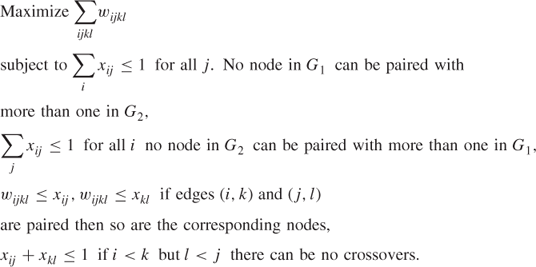
This model has 2160 constraints and 179 variables. It is not necessary to stipulate that the 80 w_ijkl variables be integer as this will be satisfied automatically. Also it is not necessary to constrain the w_ijkl to be non-negative. They can be regarded as ‘free’ variables Avoiding these two stipulations helps the model to solve more easily.