
Chapter 5
Applications and special types of mathematical programming model
5.1 Typical applications
The purpose of this section is to create an awareness of the areas where linear programming (LP) is applicable. To categorize totally those industries and problems where LP can, or cannot, be used would be impossible. Some problems clearly lend themselves to an LP model. For other problems, the use of an LP model may not provide a totally satisfactory solution but may be considered acceptable in the absence of other approaches. The decision of when to use, and when not to use, LP is often a subjective one depending on an individual's experience.
This section can do no more than try to give a ‘feel’ for those areas in which LP can be applied. In order to do this, a list of industries and areas in which the technique has been applied is given. This list is by no means exhaustive but is intended to include most of the major users. A short discussion is given of the types of LP models that are of use in each area. References are given to some of the relevant published case studies. In view of the very wide use that has been made of LP, it would be almost impossible to seek out every reference to published case studies. Nor would it be helpful to submerge the reader in a mass of often superfluous literature. The intention is to give sufficient references and allowing the reader to follow up published case studies. From the references given here, it should be possible to find other references if necessary. In many cases, practical applications are illustrated by problems in Part II.
Although the intention is mainly to consider LP applications in this chapter, the resultant models can very often naturally be extended by integer programming or non-linear programming models. In this way, more complicated or realistic situations can often be modelled. These topics and further applications are considered more fully in Chapters 7, 8, 9 and 10.
The subject of LP does not have clearly defined boundaries. Other subjects impinge on, and merge with, LP. Two types of model that have, to some extent, been studied independently of LP are considered further in this chapter. Firstly, economic models, which are sometimes referred to as input–output or Leontief models, are considered in Section 5.2. Such models can often be regarded as a special type of LP model. Secondly, network models, which arise frequently in operational research, are considered in Section 5.3. Such models are, again, often usefully considered as special types of LP model. Another area that also has connections with LP is not considered in this book in view of its limited practical applicability to date. This is the theory of games. Game theory models can sometimes be converted into LP models (and vice versa).
The following list of applications should indicate the surprisingly wide applicability of LP and, in consequence, its economic importance. Many more references exist than are given. The purpose of the references is to give a ‘window’ into the literature.
5.1.1 The petroleum industry
This is by far the biggest user of LP. Very large models involving thousands, and occasionally tens of thousands, of constraints have been built. These models are used to help make a number of decisions starting with where and how to buy crude oil, how to ship it and which products to produce out of it. Such ‘corporate models’ contain elements of distribution, resource allocation, blending and possibly, marketing. A typical example of the sort of model that arises in the industry is the REFINERY OPTIMIZATION problem of Part II. Descriptions of the use of LP in the petroleum industry are given by Manne (1956), Catchpole (1962) and McColl (1969).
5.1.2 The chemical industry
The applications here are rather similar to those in the petroleum industry although the models are rarely as large. Applications usually involve blending or resource allocation. An application is described by Royce (1970).
5.1.3 Manufacturing industry
LP is frequently used here for resource allocation. The ‘product mix’ example described in Section 1.2 is an example of this type of application. Resources to be allocated are usually processing capacity, raw materials and manpower. A multi-period problem of this type, considered in relation to the engineering industry, is the FACTORY PLANNING problem of Part II. Other common applications of LP in manufacturing are blending and blast furnace burdening (the steel industry). Three references to the application of LP here are Lawrence and Flowerdew (1963), Fabian (1967) and Sutton and Coates (1981).
5.1.4 Transport and distribution
Problems of distribution can often be formulated as LP models. Two classic examples are the transportation and transhipment problems, which are considered in Section 5.3 as they involve networks. A simple DISTRIBUTION problem of this type is presented in Part II. An extension of this problem, DISTRIBUTION 2, involves depot location as well and requires integer programming. Scheduling problems (e.g. lorries, aircraft, tankers, trains and buses) can often be tackled through integer programming. One such problem is the MILK COLLECTION problem given in Part II. Problems of assignment (trains to mines and power stations) arising in transport have also been tackled through mathematical programming. A comprehensive description of the use of mathematical programming in shipping is given in Christiansen et al. (2007). Applications of mathematical programming in distribution, in general, are described by Eilon et al. (1971) and Markland (1975).
5.1.5 Finance
A very early application of mathematical programming was in portfolio selection. This was due to Markowitz (1959). Given a sum of money to invest, the problem was how to spend it among a portfolio of shares and stocks. The objective was to maintain a certain expected rate of return from the investment but to minimize the variance of that return. The model that results is a quadratic programming model.
Agarwala and Goodson (1970) suggest how LP can be used by a government to design an optimum tax package to achieve some required aim (in particular, an improvement in the balance of payments).
LP is increasingly being used in accountancy. The economic information that can be derived from the solution to an LP model can provide accountants with very useful costing information. This sort of information is described in detail in Section 6.2. A description of how LP can be used in accountancy is given by Salkin and Kornbluth (1973).
Spath et al. (1975) describe how an LP model is applied by a mail order firm in order to minimize the total interest cost on all credits.
An interesting extension of a finance model to allow the user to set goals interactively (rather than objectives) and operate within the degrees of freedom permitted by the constraints is described by Jack (1985).
A very important potential area of application is yield (revenue) management, which is concerned with setting prices for goods at different times in order to maximize revenue. It is particularly applicable to the hotel, catering, airline and train industries. An example of its use is the YIELD MANAGEMENT problem in Part II.
5.1.6 Agriculture
LP has been used in agriculture for farm management. Such models can be used to decide what to grow where, how to rotate crops, how to expand production and where to invest. An example of such a problem is the FARM PLANNING problem of Part II. Swart et al. (1975) apply a multi-period LP model to planning the expansion of a large dairy farm. Other general references are Balm (1980) and Fokkens and Puylaert (1981).
Blending models are often applicable to agriculture problems. It is often desired to blend together livestock feeds or fertilizer at minimum cost. Glen (1980) describes a model for beef cattle ration formulation.
Distribution problems often arise in this area. The distribution of farm products, in particular milk, can be examined by the network type of LP model described in Section 5.3.
Models for planning the growth and harvesting of a number of agricultural products are described by Glen (1980, 1988, 1995, 1996, 1997).
Quadratic programming has been used for determining optimal prices for the sale of milk in the Netherlands. This is described by Louwes et al. (1963). The AGRICULTURAL PRICING problem of Part II is based on this study. A mixed integer programming model for irrigation in a developing country is described by Rose (1973).
5.1.7 Health
The obvious application of mathematical programming in this area is in problems of resource allocation. How are scarce resources, for example, doctors, nurses, hospitals, etc., to be used to best effect? In such problems, there will obviously be considerable doubt concerning the validity of the data, for example, how much of a nurse's time does a particular type of treatment really need? In spite of doubts concerning much of the data in such problems, it has been possible to use mathematical programming models to suggest plausible policy options. McDonald et al. (1974) describe a non-linear programming model for allocating resources in the UK health service. Revelle et al. (1969) describe how a non-linear programming model can be used for controlling tuberculosis in an underdeveloped country.
Warner and Prawda (1972) describe a mathematical programming model for scheduling nurses. Redpath and Wright (1981) describe how LP is used to decide intensity and direction of beams for irradiating cancerous tumours.
5.1.8 Mining
A number of interesting applications of mathematical programming occur in mining. The straightforward applications are simply ones of resource allocation, that is, how should manpower and machinery be deployed to best effect?
Blending problems also occur when it is necessary to mix together ores to achieve some required quality.
Two examples of mining problems are given in Part II. The MINING problem concerns what combination of mines a company should operate in successive years. The OPENCAST MINING problem is to decide what the boundaries of an opencast mine should be. References to the application of mathematical programming in mining are Young et al. (1963), Meyer (1969) and Boland et al. (2009).
5.1.9 Manpower planning
The possible movement of people between different types of job and its control by recruitment, promotion, retraining, etc., can be examined by linear programming. An example of such a problem, MANPOWER PLANNING, is given in Part II. Applications of mathematical programming to manpower planning are described by Price and Piskor (1972), Davies (1973), Vajda (1975), Charnes et al. (1975) and Lilien and Rao (1975).
5.1.10 Food
The food industry makes considerable use of LP. Blending (sausages, meat pies, margarines, ice cream, etc.) is an obvious application often giving rise to very small and easily solved models.
Problems of distribution also arise in this industry giving rise to the network type models described in Section 5.3.
As in other manufacturing industries, problems of resource allocation arise, which can be tackled through LP.
The FOOD MANUFACTURE problem of Part II is an example of a multi-period blending problem in the food industry. A more complicated version of this problem is described by Williams and Redwood (1974). Jones and Rope (1964) describe another LP model in the food industry.
5.1.11 Energy
The electricity and gas supply industries both use mathematical programming to deal with problems of resource allocation. The TARIFF RATES (POWER GENERATION) problem of Part II involves scheduling electric generators to meet varying loads at different times of day. This problem is similar to that described by Garver (1963). This problem is extended to the HYDRO POWER model, which illustrates another important application. Archibald et al. (1999) describe how a similar problem can be tackled by stochastic dynamic programming.
LP can also be applied to distribution problems involving the design and use of supply networks.
Applications of mathematical programming in these areas are also described by Babayer (1975), Fanshel and Lynes (1964), Muckstadt and Koenig (1977) and Khodaverdian et al. (1986).
5.1.12 Pulp and paper
Problems of resource allocation in the manufacture of paper give rise to LP models. Such models frequently involve an element of blending. In addition, the possibility of recycling waste paper has also been examined by LP as described by Glassey and Gupta (1974).
A totally different type of problem arising in the paper industry (and the glass industry) is the trimloss problem. This is the problem of arranging orders for rolls of paper of different widths so as to minimize the wastage. This problem can be tackled by linear (or sometimes integer) programming. This problem is described by Eisemann (1957). It has also been considered by Gilmore and Gomory (1961, 1963). It is used, in Section 9.6, to demonstrate column generation.
5.1.13 Advertising
The problem of spreading one's advertising budget over possible advertising outlets (television commercials, newspaper advertisements, etc.) has been approached through mathematical programming. These problems are known as media scheduling problems.
Authors differ over the usefulness of mathematical programming in tackling this type of problem. Selected references are Engel and Warshaw (1964), Bass and Lonsdale (1966) and Charnes et al. (1968). The last-mentioned reference gives a very full list of references itself.
5.1.14 Defence
Problems of resource allocation give rise to military applications of LP. Such an application is described by Beard and McIndoe (1970).
The siting of missile sites is described by Miercort and Soland (1971).
5.1.15 The supply chain
It is apparent, from the discussion of applications above, that many aspects of an organization are amenable to being modelled using mathematical programming. This is particularly true of the manufacturing industry but is also true of other industries such as finance and telecommunications. When optimizing the operations of only one aspect, or division, of an organization, one is in danger of losing sight of the ‘bigger picture’. Furthermore, there can sometimes be a danger of damaging part of an organization's operations by optimizing the operations of another part. For example, concentrating entirely on maximizing production could result in policies that are infeasible from the point of view of distribution or marketing. What are needed are integrated models that link together such different aspects. There is, of course, a danger that such models could become unwieldy and unusable if approached in the wrong way (the aborting of the projected huge IT system for the British National Health Service is a stark reminder). Such major considerations form the subject of information systems and are beyond the scope of this book. It is usually the case that such integrated models evolve from existing models of smaller specialist functions. Some of the discussion in Chapter 4 is relevant to this. Advances in information technology, for example, communications software, database technology and ‘user-friendly’ interfaces have made it easier to create and use such models.
Although applicable in other areas, we illustrate our discussion of supply chain models by using examples from the manufacturing sector. The following functions are amenable to optimization:
In addition other, non-mathematical programming models may be relevant, for example, forecasting and accounting models.
A supply chain model integrates models for all, or some, of these functions, taking outputs from some as inputs to others, and performs a global optimization, for example, to maximize total profit.
5.1.16 Other applications
There are numerous other applications of mathematical programming. A few of the less usual ones are given here as they might otherwise go unnoticed.
Heroux and Wallace (1973) describe a multi-period LP model for land development.
Souder (1973) discusses the effectiveness of a number of mathematical programming models for research and development. Feuerman and Weiss (1973) show how a knapsack integer programming model can be used to help design multiple choice–type examinations. Kalvaitis and Posgay (1974) apply integer programming to the problem of selecting the most promising kind of mailing list.
Wardle (1965) applies LP to forestry management.
Problems of pollution control have been tackled through mathematical programming. Applications are described by Loucks et al. (1968).
Kraft and Hill (1973) describe a 0–1 integer programming model for selecting journals for a university library.
Jünger et al. (1989) and Ferreira et al. (1993) describe integer programming models arising in computer design.
Bollapragada et al. (2001) apply integer programming to the civil engineering problem of truss design, that is, constructing an optimal structure of trusses to support a given weight, modelling the logical dependencies of trusses.
Trick has applied integer programming extensively to sports scheduling (see, e.g. Nemhauser and Trick (1998)).
Chang and Sahinidis (2011), among others, have applied integer programming to DNA sequencing. This has similarities to the (easier) archaeological seriation problem, which has been considered by Laporte (1976) and Wilkinson (1971), who formulate this problem as a version of the Travelling Salesman Problem (see Chapter 9).
The use of LP for performance evaluation in a number of organizations (particularly in the public sector) through the use of a type of model known as Data Envelopment Analysis has become important. This is described through the EFFICIENCY ANALYSIS problem in Part II. References are Charnes et al. (1978), Farrell (1957), Land (1991) and Thanassoulis et al. (1987).
A much fuller list of papers on mathematical programming applications has been compiled by Riley and Gass (1958). The special editions of the journal Mathematical Programming Studies Nos 9 (1975) and 20 (1982) are devoted to applications.
5.2 Economic models
A widely used type of national economic model is the input–output model representing the interrelationships between the different sectors of a country's economy. Such models are often referred to as Leontief models after their originator, who built such a model of the American economy. This is described by Leontief (1951). Input–output models are often regarded usefully as a special type of LP model.
5.2.1 The static model
The output from a particular industry or a sector of an economy is often used for two purposes: (i) for immediate consumption, for example, coal to be sold to domestic consumers; (ii) as an input to other industries or sectors of the economy, for example, coal to provide power for the steel industry. As the outputs from many industries can be split in this way between (exogenous) consumption and as (endogenous) inputs into these same industries, a complex set of interrelationships will exist. The input–output type of model provides about the simplest way of representing these relationships. A number of strong (and usually oversimplified) assumptions are made regarding the inter-industry relationships. The two major assumptions are as follows:
In order to demonstrate such a model, we will consider a very simple example.
Table 5.1 An input–output matrix
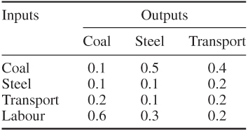
| Coal | 20 |
| Steel | 5 |
| Transport | 25 |
5.5 ![]()
![]()
![]()
The model described above is unrealistic in a number of respects. Equations (5.4)–(5.6) give no real limitation to the productive capacity of the economy. It can fairly easily be shown that so long as a particular, positive, bill of goods can be produced (the economy is a ‘productive’ one), then these relationships guarantee that any bill of goods, however large, can be produced. This is clearly unrealistic. Firstly, we would expect some limitation on productive capacity preventing more than a certain amount of output from each industry in a given period of time. Secondly, we would expect the output from an industry only to be effective as the input to another industry after a certain time has elapsed. This second consideration leads to dynamic input–output models, which we consider below. Before doing this, however, we will consider the problem of modelling limited productive capacity in the case of a static model.
In our small example, we assumed that once we had decided how much each industry should produce in order to meet a specified bill of goods, we could provide the labour required. If labour were in short supply, it might limit our productive capacity. There would then be interest in seeing what bills of goods are or are not producible in a particular period of time. Returning to our example, if we were to limit labour to 40 (£m per year) we could not produce our previous bill of goods. But what bill of goods could we produce? Answers to this question can be explored through LP. Variables will now represent our bill of goods:
| Coal | yc |
| Steel | ys |
| Transport | yt |
Equations (5.4)–(5.6) will give the constraints
5.8 ![]()
5.9 ![]()
The labour limitation gives the constraint
Achievable bills of goods will be represented by the values of yc, yr and yt in feasible solutions to Equations (5.7)–(5.10). Specific solutions can be found by introducing an objective function. For example, we might wish to maximize the total output:
5.11 ![]()
Alternatively, we might weight some outputs more heavily than others by giving xc, xs and xt different objective coefficients. We might wish simply to maximize production in one particular sector of the economy, such as steel, and simply maximize xs. This is clearly a situation of the type referred to in Section 3.2 in which it is of interest to experiment with a number of different objectives rather than simply concentrate on one.
We have considered only labour as a limiting factor in productive capacity. In practice, there could well be other resource limitations such as processing capacity, raw material, etc. Such limitations could, of course, easily be incorporated in a model by extra constraints. Limited resources of this sort are sometimes known as primary goods. Primary goods only provide inputs to the economy. They are not produced as outputs as well. A major advantage of treating such models as LP models is that a lot of subsidiary economic information is also obtained from solving such a model. Such information is described very fully in Section 6.2. In particular, valuations are obtained for the constraints of a model. These valuations are known as shadow prices. For the type of model considered here, we would obtain meaningful valuations for the primary goods. In this way, a pricing system could be introduced into our model. This would give suitable prices for the outputs from all the industries.
Although any number of primary goods can be considered in an LP formulation of an input–output model, it is quite common only to consider labour. In practice, particularly in the relatively simple economies of developing countries, it may well not be unreasonable to consider labour as the overall limitation. If this can be done, there is another less obvious advantage to be gained in the applicability of such a model. It has already been pointed out that an input–output model assumes non-substitutability of the inputs, that is, it is not possible to vary the relative proportions in which all the inputs are used to produce the output of a particular industry. In practice, this might well be a far from realistic assumption. For example, we might well be able to produce each unit of coal by using more power (more coal) and less machinery (less steel). To model this possibility would require a variation in the coefficients of the input–output matrix. It has been shown that if there is only one primary good (usually labour), then it will only be worthwhile to concentrate on one production process for each industry. This is the result of the Samuelson substitution theorem, which we will not prove. Such theoretical results and a fuller description of input–output models are given in Dorfman et al. (1958). Another good reference is Shapiro (1979). The importance of this result is that we need not worry about the apparent non-substitutability limitation so long as we only have one primary good. There will be one, and only one, best set of inputs (production processes) for each industry. This best production process will remain the best no matter what bill of goods we are producing. There is, of course, the problem of finding, for each industry, the production process which should be used. Once, however, this has been done, no matter what the bill of goods, we need only incorporate this one production process (column of the input–output matrix) into all future models. In fact, the finding of the best production process for each industry can be done by LP. To illustrate how this may be done as well as illuminating the import of the Samuelson substitution theorem, we will extend our small example. Table 5.2 gives two possible sets of inputs (production processes) to produce 1 unit of the three industries.
Table 5.2 An input–output matrix with alternative production processes
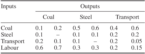
In practice, there might be many more (possibly an infinite number) than two processes for each industry.
On the face of it, we might think it advantageous to use some combination of the two processes for producing coal. The first process is more economical on coal but uses some steel as well, which the second process does not. Similarly, some mixture of the two processes for producing steel and the two processes for producing transport might seem appropriate. Moreover, which processes are used might seem likely to depend upon the particular bill of goods.
We repeat, however, that our intuitive idea would be false. There will be exactly one best process for each industry and this will be used whatever bill of goods we have. Instead of the variables xc, xs and xt in our original model we can introduce variables xc1, xc2, xs1, xs2, xt1 and xt2 to represent the total quantities of coal, steel and transport produced by each process. Using the same bill of goods as before, instead of constraints (5.1)–(5.3), we obtain
5.12 ![]()
5.13 ![]()
5.14 ![]()
These equations can be written as
5.16 ![]()
5.17 ![]()
We are considering labour as the only primary good and will limit ourselves to 60 (£m). This gives the constraint
There will generally be more than one solution to a system such as this. In order to find the ‘best’ solution we will define an objective function. One possible objective function would, of course, be to ignore constraint (5.18) and minimize the expression on the left-hand side representing labour usage. Alternatively, we might specify another objective function. For this example, we will do this and simply maximize total output:
Our resultant optimal solution gives
Notice that the Samuelson substitution theorem has worked in this case. One process in each industry is the best to the total exclusion of all the others. Moreover, it could be shown that these processes will be the best no matter what the bill of goods is. The optimal solution will be made up of only the variables xc1, xs1 and xt2, no matter what the right-hand side coefficients in constraints (5.15)–(5.18) are. We could, therefore, confine all our attention to these processes and ignore the others. It should be noted, however, that these ‘best’ processes are only the best because of the objective function (5.19) that we have chosen. If instead of maximizing output, we were to choose another objective, it might be preferable to switch to another process in some cases. It will never, however, be worth ‘mixing’ processes. Once we consider more than a single primary good such mixing may well, however, become desirable.
5.2.2 The dynamic model
We have pointed out that our static model assumed that we could ignore time lags between an output being produced and used as an input to another (or the same) industry. This unrealistic assumption can be avoided by introducing a dynamic model. It has already been shown in Section 4.1 that LP models can often be extended to multi-period models. We can do much the same thing with the static type of input–output model. In practice, some of the output from an economy will immediately be consumed (e.g. cars for private motoring) while some will go to increase productive capacity (e.g. factory machinery). Such alternative uses for the output will result in different possible growth patterns for the economy, that is, we can live well now but neglect to invest for the future or we can sacrifice present day consumption in the interests of future wealth-producing capacity. A simple example of such a problem, ECONOMIC PLANNING, leading to a dynamic input–output model is given in Part II. Rather than discuss Dynamic input–output models, the discussion is taken up with the formulation of this problem in Part III. A description of dynamic input–output models of this type is given by Wagner (1957).
5.2.3 Aggregation
To sum up the characteristics of a whole industry or sector of an economy in one column of an input–output matrix obviously requires a large amount of simplification of the real situation. It is necessary to group together many different industries into one. This aggregation is necessary in order to obtain a reasonable size of problem. Most input–output models are aggregated into less than 1000 industries. The problem of aggregation is obviously of paramount concern to the model builder. Unfortunately, very little theoretical work has been done to indicate mathematically when aggregation is and is not justified. Three criteria that common sense would suggest to be good grounds for aggregating particular industries are (i) substitutability, (ii) complementarity and (iii) similarity of production processes. Problems of this sort are discussed more fully by Stone (1960).
In view of their sophistication and efficiency, commercial mathematical programming packages provide a useful way of solving input–output models. Even if the model is of the simplest kind described above and only requires the solution of a set of simultaneous equations, such packages are of use. Almost all packages contain an inversion routine, which is very useful for inverting large matrices (sets of simultaneous equations). It should, however, be pointed out that input–output models are often quite dense. In this respect, they are untypical of general LP models. As already mentioned in Section 2.12.1, in a model with 1000 constraints, one would expect only about 1% of the coefficients to be non-zero. For an input–output model, this figure could well be as high as 50%. As a result, input–output models can take a long time to solve on a computer and run into numerical difficulties. It is sometimes worth exploiting the special structure of an input–output LP model and using a special purpose algorithm. Dantzig (1955) describes how the simplex algorithm can be adapted to this purpose.
5.3 Network models
The use of models involving networks is very widespread in operational research. Problems involving distribution, assignment and planning (critical path analysis and PERT) frequently give rise to the analysis of networks. Many of the resultant problems can be regarded as special types of LP problem. It is often more efficient to use special purpose algorithms rather than the revised simplex algorithm. Nevertheless, it is important for the model builder to be aware when he/she is dealing with a special kind of LP model. In order to solve the model it may be useful for the builder to adapt the simplex algorithm to suit the special structure. It may even, sometimes, be worth ignoring the special structure and using a general purpose package program. As such programs are often highly efficient and well-designed, their speeds outweigh the algorithmic efficiency of less well-designed but more specialized programs.
It is not intended that the coverage of this topic be comprehensive. The main aim is simply to show the connection between network models and LP models. References are given to much fuller treatments of the subject.
5.3.1 The transportation problem
This famous type of problem first described by Hitchcock (1941) is usefully regarded as one of obtaining the minimum cost flow through a special type of network.
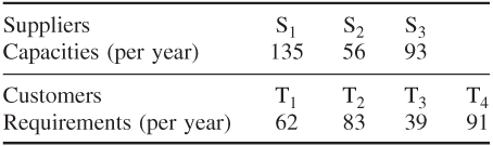
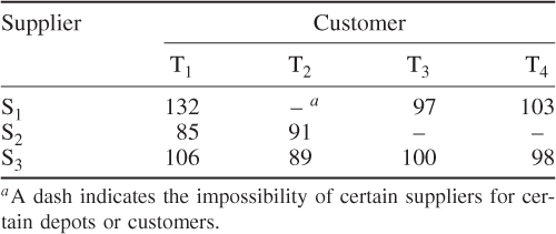
Suppose that a number of suppliers (S1, S2, …, Sm) are to provide a number of customers (T1, T2, …, Tn) with a commodity. The transportation problem is how to meet each customer's requirement, while not exceeding the capacity of any supplier, at minimum cost. Costs are known for supplying 1 unit of the commodity from each Si to each Tj. In some cases, it may not be possible to supply a particular customer Tj from a particular supplier Si. It is sometimes useful to regard these costs as infinite in such cases. In distribution problems, these costs will often be related to the distances between Si and Tj. It is assumed that the capacity of each supplier (over some period such as a year) is known and the requirement of each customer Tj is also known. In order to describe the problem further, we will consider a small numerical example.
5.20 ![]()
5.22 ![]()
5.25 ![]()
5.26 ![]()
5.28 ![]()
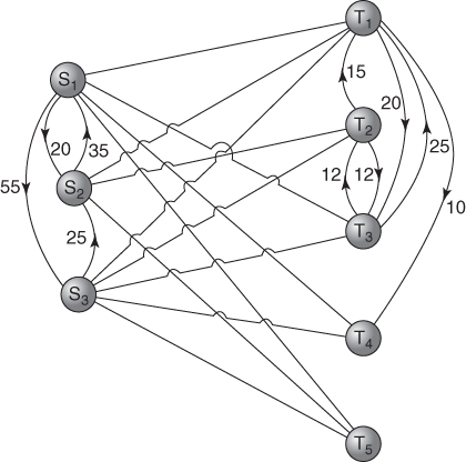
The above problem can be looked at graphically as illustrated in Figure 5.1.
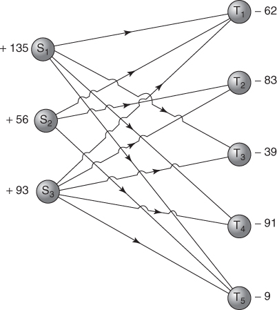
In the network of Figure 5.1, we have the suppliers S1, S2 and S3 and the five customers T1, T2, T3, T4, and T5 (including the dummy customer). Si and Tj provide the nodes of the network to which we have attached the (positive) capacities or (negative) requirements. The possible supply patterns Si to Tj provide the arcs of the network to which we have attached the unit supply costs. Our problem can now be regarded more abstractly as one where we wish to obtain the minimum cost flow through the network. The Si nodes are ‘sources’ for the flow entering the system and the Tj nodes are ‘sinks’ where flow leaves the system. We must ensure that there is continuity of flow at each node (total flow in equals total flow out). These conditions give rise to material balance constraints of the type discussed in Section 3.3.
If xij represents the quantity of flow in the arc i to j we obtain the following constraints:
5.28 ![]()
5.29 ![]()
5.30 ![]()
5.31 ![]()
5.32 ![]()
5.33 ![]()
5.34 ![]()
These constraints are clearly equivalent to the constraints (5.21) to (5.27). We have, however, added the dummy customer T5. This has resulted in the additional variables x15, x25 and x35, and an added constraint (5.35), but allowed us to deal entirely with ‘=’ constraints. We have also revised the signs on both sides of the availability constraints. For more general minimum cost flow problems, which we consider later, it is convenient to give negative coefficients to flows out of a node and positive coefficients to flows in. Therefore, this convention has been applied here.
The transportation problem also arises in less obvious contexts than distribution. We give a numerical example below of a production planning problem.
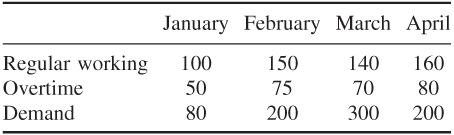
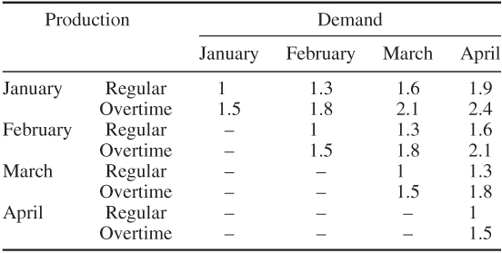
Transportation problems are obviously expressed much more compactly in a square array such as Tables 5.3 and 5.4 rather than as an LP matrix. This is one virtue of using a special purpose algorithm. Dantzig (1951) uses the simplex algorithm but works within this compact format. The special structure results in the algorithm taking a particularly simple form. An alternative algorithm for the transportation problem is due to Ford and Fulkerson (1956). This algorithm is usefully thought of as a special case of a general algorithm for finding the minimum cost flow through a network. Such problems are considered below and described in Ford and Fulkerson (1962).
As a result of their special structure, transportation problems are particularly easy to solve in comparison with other LP problems of comparable size. They also have (together with some other network flow problems) the very important property that so long as the availabilities and requirements at the sources and sinks are integral, the values of the variables in the optimal solution will also be so. For example, so long as the right-hand side coefficients in the constraints (5.21)–(5.27) of the LP problem of Example 5.2 are integers, the variable values in the optimal solution will be as well. This rather surprising property of the transportation problem is computationally very important in many circumstances as it avoids the necessity of using integer programming to ensure that variables take integer values. As will be discussed in Chapters 8, 9 and 10, integer programming models are generally much more difficult to solve than LP models.
Sufficient conditions for a model to be expressible as a network flow problem are discussed in Section 10.1. The recognition of such conditions is important as it allows the use of specialized efficient algorithms and avoids the use of computationally expensive integer programming.
A further constraint that sometimes applies to transportation problems is that there are limits to the possible flow from a source to a sink. This gives rise to the capacitated transportation problem. There may be both lower and upper limits for the flow in each arc. For the LP formulation of the transportation problem (such as exemplified in Example 5.2 above) such limits can be accommodated by simple bounds on the variables:
![]()
Frequently, lij will be 0. Capacitated transportation problems can, like the ordinary transportation problem, be solved by straightforward extensions to the special purpose algorithms mentioned above.
Another non-distribution example of the transportation problem is described by Stanley et al. (1954), who describe how the problem arises in deciding how a government should award contracts.
5.3.2 The assignment problem
This is the problem of assigning n people to n jobs so as to maximize some overall level of competence. For example person i might take an average time tij to do job j. In order to assign each person to a job and to fill each job so as to minimize total time for all tasks our problem would be

where
This can obviously be regarded as a special case of the transportation problem. We can regard it as a problem with n sources and n sinks. Each source has an availability of 1 unit and each sink has a demand of 1 unit. Constraints (5.36) impose the condition that each job be filled. Constraints (5.37) impose the condition that every person be assigned a job.
It might appear that this problem demands integer programming in order to ensure that xij can only take the values 0 or 1. Fortunately, however, because this problem is a special case of the transportation problem the integrality property mentioned above holds. If we solve an assignment problem as a conventional LP model, we can be certain that the optimal solution will give integer values to the xij (0 or 1). If marriage is regarded as an assignment problem of this kind, Dantzig has suggested that the integrality property shows that monogamy leads to greatest overall happiness!
Obviously assignment problems could be solved as LP models, although the resultant models could be very large. For example, the assigning of 100 people to 100 jobs would lead to a model with 10 000 variables. It is much more efficient to use a specialized algorithm. One of the specialized algorithms for the transportation problem could obviously be applied. The most efficient method known is one allied to the Ford and Fulkerson algorithm but more specialized. This is known as the Hungarian method and is described by Kuhn (1955).
5.3.3 The transhipment problem
This is an extension of the transportation problem, due to Orden (1956). In this problem, it is possible to distribute the commodity through intermediate sources and through intermediate sinks as well as from sources to sinks. In Example 5.2, we could allow flow (at a certain cost) between suppliers S1, S2 and S3 as well as between customers T1, T2, T3 and T4. It might be advantageous sometimes to send a commodity from one supplier to another before dispatching it to the customer. Similarly, it might be advantageous to send a commodity to a customer via another customer first. The transhipment problem allows for these possibilities.
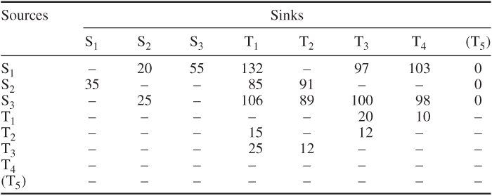
If we extend Example 5.2 to allow the use of certain intermediate sources and sinks, our graphical representation would be of the form of Figure 5.2.
Costs have now been attached to the arcs between sources and the arcs between sinks. Notice that it is sometimes possible to go either way between sources (or sinks), at not necessarily the same cost.
It is possible to convert a transhipment problem into a transportation problem. To do this, the sources and sinks are considered firstly as being all sources and then as all sinks. When considered as sinks, sources have no availabilities, and when considered as sources, sinks have no requirements. Flow from a sink to a source is not allowed. For the transhipment extension of Example 5.2 illustrated in Figure 5.2, we can draw up the unit cost array of Table 5.5. ‘Sources’ T1, T2, T3 and T5will have zero availabilities and ‘sinks’ S1, S2 and S3 zero requirements.
Transhipment problems can obviously be formulated as LP models just as the transportation problem can. Again, it is often desirable to use a specialized algorithm such as that described by Dantzig (1951) or by Ford and Fulkerson (1962).
As with transportation problems, transhipment problems can be extended to capacitated transhipment problems where the arcs have upper and lower capacity limitations. These can also be solved by specialized algorithms.
An application of the transhipment problem outside the field of distribution is described by Srinivason (1974).
5.3.4 The minimum cost flow problem
The transportation, transhipment and assignment problems are all special cases of the general problem of finding a minimum cost flow through a network. Such problems may have upper and lower capacities attached to the arcs in the capacitated case. The uncapacitated case will be considered here.
![]()
5.39 ![]()
5.41 ![]()
5.42 ![]()
5.43 ![]()
5.44 ![]()
As with the other types of model so far discussed in this section, it is generally more efficient to use specialized algorithms. Those due to Dantzig (1951) and Ford and Fulkerson (1962) are also applicable here.
A comprehensive survey of applications of the minimum cost network flow problem is given by Bradley (1975). Other useful references are Glover and Klingman (1977) and Jensen and Barnes (1980).
It is sometimes possible to convert an LP model into a form that is immediately convertible into a network flow model. A procedure for doing this, or showing such a conversion to be impossible, is given in Section 5.4.
If arcs have lower or upper bounds (or both) on their capacities, then (as with the special case of the transportation problem) it is possible to adapt the special algorithms to cope with this. It is, however, worth pointing out that such models can be converted to the uncapacitated case. This might be necessary if a program was being used which could not deal with such bounds.
Suppose the flow from node i to node j had a lower bound of l (and cost cij). An extra node i′ can be added with a new arc from i to i′. If there is an external flow l out of i and into i′, as shown in Figure 5.4, this provides the necessary restriction. Similarly, Figure 5.5 demonstrates how an upper bound of u can be imposed on the flow in arc i − j.

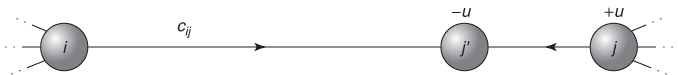
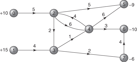
It is important to ensure that a minimum cost network flow problem is well defined. For example the unit flow costs are generally non-negative. If negative costs are allowed it is important to ensure that cost cannot be minimized indefinitely (giving an unbounded problem). This could happen, for example, if arc 2–4 were given in a unit cost of −6 instead of +6. Going round the loop indefinitely would continuously reduce the cost.
A minimum cost network flow problem, DISTRIBUTION, is given in Part II.
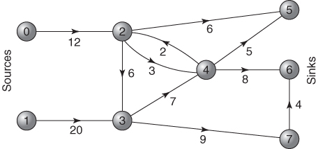
An extension of the problem of finding the minimum cost flow of a single commodity through a network is the problem of minimizing the cost of the flows of several commodities through a network. This is the minimum cost multi-commodity network flow problem. There will be capacity limitations on the flows of individual commodities through certain arcs as well as capacity limitations on the total flow of all commodities through individual arcs. For example, in the network of Figure 5.3, one commodity might flow between source 0 and sink 5 and a second commodity flow between source 1 and sinks 6 and 7. This type of problem can again be formulated as an LP model. The resultant model has a block angular structure of the type discussed in Section 4.1. The block angular structure makes the decomposition procedure of Dantzig and Wolfe, which is discussed in Section 4.2, applicable. In fact this leads to another LP formulation of the problem. This aspect of the minimum cost multi-commodity network flow problem is discussed by Tomlin (1966).
Apart from decomposition there are no special algorithms applicable to the general minimum cost multi-commodity network flow problem. The (often large) LP model resulting from such a problem is best solved by the standard revised simplex algorithm using a package programme.
Charnes and Cooper (1961a) formulate a traffic flow problem as a minimum cost multi-commodity network flow model.
This extension of the single-commodity network flow LP model to more than one commodity destroys the property that guarantees an integral optimal solution. Fractional values for the flows may result from the optimum solution to the LP model even if all capacities, availabilities and requirements are integral. If the nature of the problem requires an optimal integer solution it is necessary to resort to integer programming.
Another important extension of the minimum cost network flow model is the generalized network flow model. This is sometimes known as the network flow with gains model. In this extension, the flow in an arc may alter between the two nodes. A multiplier is then associated with each arc, which gives the factor by which flow is altered. Situations that require this modification result from, for example, evaporation, wastage or application of interest rates. Glover and Klingman (1977) give applications. If it is necessary that the flows be integer values, then this can no longer be guaranteed from an LP solution. It is necessary to use integer programming methods. Nevertheless, it is possible to exploit this simple structure to good effect in the algorithms used. Glover et al. (1978) describe such a method. In fact, any 0–1 integer programming problem can be converted into such a generalized network model where flows must be integer values. This is shown by Glover and Mulvey (1980).
5.3.5 The shortest path problem
This is the problem of finding a shortest path between two nodes through a network. Rather surprisingly, this problem can be regarded as a special case of the minimum cost flow problem.
Although it is possible to use conventional LP to solve shortest path problems it would be more efficient to use a specialized algorithm. One of the most efficient such algorithms is due to Dijkstra (1959).
5.3.6 Maximum flow through a network
When a network has capacity limitations on the flow through arcs there is often interest in finding the maximum flow of some commodity between sources and sinks. We will again consider the network of Example 5.4 but our objective will now be to maximize the flows into the sources and out of the sinks rather than these quantities being given. Each arc has now been given an upper capacity, which is the figure attached to it in Figure 5.7.
5.46 
5.47 ![]()
5.48 ![]()
5.49 ![]()
5.50 ![]()
5.51 ![]()
5.52 ![]()
5.53 ![]()
![]()
Again, this type of model has the property that the optimal solution will give integer flows so long as the capacities are integer.
It is again more efficient to use a specialized algorithm for this type of problem. Such an algorithm is described by Ford and Fulkerson (1962).
5.3.7 Critical path analysis
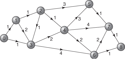
This is a method of planning projects (often in the construction industry) that can be represented by a network. The arcs of the network represent activities occupying a duration of time, for example, building the walls of a house, and the nodes are used to indicate the termination and beginning of activities. Once a project has been represented by such a network model the network can be analysed to answer a number of questions such as
Such a mathematical analysis of this kind of network is known as critical path analysis. The arcs for those activities in the network that cannot be delayed without affecting the overall completion time of the project can be shown to lie on a path. This critical path is in fact the longest path through the network. The problem of finding the critical path is a special kind of LP problem although the special structure of the problem makes a specialized algorithm appropriate.
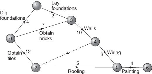
| t0 | start time for activities 0–1, 0–3 and 0–2 |
| t1 | start time for activity 1–3 |
| t2 | start time for activity 2–5 |
| t3 | start time for activity 3–4 |
| t4 | start time for activities 4–2 and 4–5 |
| t5 | start time for activity 5–6 |
| z | finish time for the project. |
5.54 ![]()
5.55 ![]()
5.56 ![]()
5.58 ![]()
5.59 ![]()
5.60 ![]()
5.61 ![]()
Building and conventionally solving the above LP model would be an inefficient method of finding the critical path. Special algorithms exist and there are widely used package programs for doing critical path analysis. Many extensions of the problem of scheduling a project in this way can be considered but are beyond the scope of this book. A full discussion of this subject is contained in Lockyer (1967).
One very practical extension of the problem is that of allocating resources to the activities in a project network. For example, in the network of Figure 5.8 both activity 4–5 (wiring) and activity 2–5 (roofing) may require people (although in this contrived example they would probably have different skills). If activity 4–5 requires three people and activity 2–5 requires six and there are only eight available, the optimal schedule given above is unattainable and one of those activities will have to be delayed or extended. The problem is then how to reschedule to achieve some objective. For example, the objective might well be to delay the overall completion time as little as possible. Alternatively, there might be a desire to ‘smooth’ the usage of this and other resources over time. This extension to the problem is mentioned again in Section 9.5 as it gives rise to an integer programming extension to the LP problem of the type above. Nevertheless, integer programming would be generally far too costly in computer time to justify solving this type of problem in this way. A problem that gives rise to a very simple network is job-shop scheduling. This problem of scheduling jobs on machines can be regarded as a problem of allocating resources to activities in a network. The operations in the job-shop (e.g. machining) give the activities. Sequencing relations between those operations give a (simple) network structure. The resources to be allocated are the limited machines.
All the problems described in this section (apart from the minimum cost multi-commodity network flow problem) are best tackled through specialized algorithms rather than the revised simplex algorithm available on commercial package programs. The reason for describing these problems and showing how they can, if necessary, be modelled as linear programs is that many practical problems are made up, in part, of network problems. Such problems often, however, contain additional complications that make it impossible to use a pure network model. This is where the conventional LP formulation becomes important. Many practical LP models have a very large network component. Such a feature usually makes very large models easy to solve using package programs. Some package programs have special features to take advantage of some of the network structure within a model. An example of this is the generalized upper bound (GUB) type of constraint, which was mentioned in Section 3.3. In the LP formulation of the transportation problem in Example 5.2 constraints (5.21)–(5.23) could be regarded as GUB constraints and not explicitly represented as constraints if a package with this facility was used. Alternatively (and preferably because there are more of them), constraints (5.24)–(5.27) could be represented as GUB constraints. The use of the GUB facility makes the solution of many network flow problems (or problems with a network flow component) particularly easy by conventional LP.
Another virtue in recognizing a network flow component in an LP model is that many variables are likely to come out at integer values in the optimal solution. It has been pointed out that this happens for all the variables in most of the network flow problems described in this section so long as the right-hand side coefficients are integers. If a model is ‘not quite’ of a network flow kind it is probable that the great majority of variables will still take integer values in the optimal LP solution. The computational difficulties of forcing all these variables to be integer values by integer programming will be much reduced. This topic is discussed much more fully in Chapter 10.
There is also great virtue to be gained from remodelling a problem in order to get it into the form of a network flow model. This then opens up the possibility of using a special purpose algorithm. An example of how this can sometimes be done for a practical problem is given by Veinott and Wagner (1962). Dantzig (1969) shows how a hospital admissions scheduling program can be remodelled to give an LP model with a large network flow component. He then exploits this structure by use of the GUB facility. Other examples of reformulations into network flow models are Daniel (1973), Wilson and Willis (1983) and Cheshire et al. (1984).
An automatic way of either converting an LP model to a network flow model or showing such a conversion to be impossible is given in Section 5.4. The recognition or conversion of a model as a network structure relieves the need to use the computationally much more costly methods of integer programming.
In Section 6.2, the concept of the dual of an LP model is described. Every LP model has a corresponding model known as the dual model. The optimal solution to the dual model is very closely related to the optimal solution of the original model. In fact the optimal solution to either one can be derived very easily from the optimal solution to the other. It turns out that many practical problems give rise to an LP model that is the dual of a network flow model. In such circumstances, it could well be worth using a specialized algorithm on the corresponding network flow model. Moreover, the dual of any of the types of network flow mode mentioned here (apart from the minimum cost multi-commodity network flow model) also has the property of guaranteeing optimal integer solutions (so long as the objective coefficients of the original model are integers). The recognition of this type of model can, again, be of great practical importance for this reason. This topic is further discussed in Sections 10.1 and 10.2.
In Part II, the OPENCAST MINING problem can be formulated as the dual of a network flow problem. The formulation is discussed in Part III. The MINING problem of Part II can be formulated as an integer programming model, a large proportion of which is the dual of a network flow model. Some examples of such models are given in Williams (1982).
One famous network problem that has not been discussed in this section is the travelling salesman problem. This is the problem of finding a minimum distance (cost) route round a given set of cities. This problem cannot generally be solved by an LP model, in spite of its apparent similarity to the assignment problem. It can, however, be modelled as an integer programming extension to the assignment problem and is fully discussed in Section 9.5.
5.4 Converting linear programs to networks
The advantages of converting linear programs to minimum cost network flow models, if possible, have already been discussed in Section 5.3. They are further discussed in Section 10.1 as minimum cost network flow models have integer optimal solutions (so long as external flows in and out are integer values). This relieves the need to use the much more expensive procedures of integer programming.
We outline a method described by Baston et al. (1991) for converting linear programs to network flow models. Another procedure, but expressed in the more abstract language of matroid theory, is given by Bixby and Cunningham (1980).
In order to illustrate the method, we will take a numerical example.
As the conversion does not depend on the objective or right-hand side coefficients, we give these in a general form. In this example, we assume all the original constraints were of the ‘≤’ form and that slack variables have been added to make them equations. For ‘≤’ constraints surplus variables would be subtracted. If any of the original constraints were equations then we would add artificial variables (variables constrained to take the value zero). These logical (slack, surplus or artificial) variables will represent arcs in the network created. For the case of artificial variables, these arcs will finally be deleted.
We carry out the following transformations:
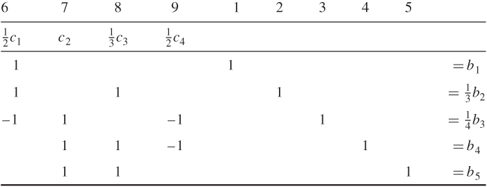
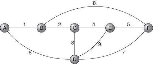
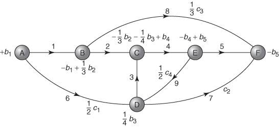
In the example, in Figure 5.10, node C has tree-arc 4 leaving it (row 4 has scaled right-hand side b4) and tree-arcs 2 and 3 entering it (rows 2 and 3 have scaled right-hand sides of (1/3)b2 and (1/4)b3, respectively). Hence the external flow into node C is b4 − (1/3)b2 − (1/4)b3. (A negative external flow would, of course, be regarded as a positive flow out.) The other nodes have external flows calculated in a similar manner.
The resulting directed network with its external flows gives the required minimum cost network flow model equivalent to the original linear program. When solved the values of the flows in the arcs may have to be unscaled according to the scaling factors applied.