
Chapter 1
Introduction
1.1 The concept of a model
Many applications of science make use of models. The term ‘model’ is usually used for a structure that has been built with the purpose of exhibiting features and characteristics of some other objects. Generally, only some of these features and characteristics will be retained in the model depending upon the use to which it is to be put. Sometimes, such models are concrete, as is a model aircraft used for wind tunnel experiments. More often, in operational research, we will be concerned with abstract models. These models will usually be mathematical in that algebraic symbolism will be used to mirror the internal relationships in the object (often an organization) being modelled. Our attention will mainly be confined to such mathematical models, although the term ‘model’ is sometimes used more widely to include purely descriptive models.
The essential feature of a mathematical model in operational research is that it involves a set of mathematical relationships (such as equations, inequalities and logical dependencies) that correspond to some more down-to-earth relationships in the real world (such as technological relationships, physical laws and marketing constraints).
There are a number of motives for building such models:
It is important to realize that a model is really defined by the relationships that it incorporates. These relationships are, to a large extent, independent of the data in the model. A model may be used on many different occasions with differing data, for example, costs, technological coefficients and resource availabilities. We would usually still think of it as the same model even though some coefficients have been changed. This distinction is not, of course, total. Radical changes in the data would usually be thought of as a change in the relationships and therefore the model.
Many models used in operational research (and other areas such as engineering and economics) take standard forms. The mathematical programming type of model that we consider in this book is probably the most commonly used standard type of model. Other examples of some commonly used mathematical models are simulation models, network planning models, econometric models and time series models. There are many other types of model, all of which arise sufficiently often in practice to make them areas worthy of study in their own right. It should be emphasized, however, that any such list of standard types of model is unlikely to be exhaustive or exclusive. There are always practical situations that cannot be modelled in a standard way. The building, analysing and experimenting with such new types of model may still be a valuable activity. Often, practical problems can be modelled in more than one standard way (as well as in non-standard ways). It has long been realized by operational research workers that the comparison and contrasting of results from different types of model can be extremely valuable.
Many misconceptions exist about the value of mathematical models, particularly when used for planning purposes. At one extreme, there are people who deny that models have any value at all when put to such purposes. Their criticisms are often based on the impossibility of satisfactorily quantifying much of the required data, for example, attaching a cost or utility to a social value. A less severe criticism surrounds the lack of precision of much of the data that may go into a mathematical model; for example, if there is doubt surrounding 100 000 of the coefficients in a model, how can we have any confidence in an answer it produces? The first of these criticisms is a difficult one to counter and has been tackled at much greater length by many defenders of cost–benefit analysis. It seems undeniable, however, that many decisions concerning unquantifiable concepts, however, they are made, involve an implicit quantification that cannot be avoided. Making such a quantification explicit by incorporating it in a mathematical model seems more honest as well as scientific. The second criticism concerning accuracy of the data should be considered in relation to each specific model. Although many coefficients in a model may be inaccurate, it is still possible that the structure of the model results in little inaccuracy in the solution. This subject is mentioned in depth in Sections 4.2 and 6.3.
At the opposite extreme to the people who utter the above criticisms are those who place an almost metaphysical faith in a mathematical model for decision-making (particularly if it involves using a computer). The quality of the answers that a model produces obviously depends on the accuracy of the structure and data of the model. For mathematical programming models, the definition of the objective clearly affects the answer as well. Uncritical faith in a model is obviously unwarranted and dangerous. Such an attitude results from a total misconception of how a model should be used. To accept the first answer produced by a mathematical model without further analysis and questioning should be very rare. A model should be used as one of a number of tools for decision-making. The answer that a model produces should be subjected to close scrutiny. If it represents an unacceptable operating plan, then the reasons for unacceptability should be spelled out and if possible incorporated in a modified model. Should the answer be acceptable, it might be wise only to regard it as an option. The specification of another objective function (in the case of a mathematical programming model) might result in a different option. By successive questioning of the answers and altering the model (or its objective), it should be possible to clarify the options available and obtain a greater understanding of what is possible.
1.2 Mathematical programming models
It should be pointed out immediately that mathematical programming is very different from computer programming. Mathematical programming is ‘programming’ in the sense of ‘planning’. As such, it need have nothing to do with computers. The confusion over the use of the word ‘programming’ is widespread and unfortunate. Inevitably, mathematical programming becomes involved with computing as practical problems almost always involve large quantities of data and arithmetic that can only reasonably be tackled by the calculating power of a computer. The correct relationship between computers and mathematical programming should, however, be understood.
The common feature that mathematical programming models have is that they all involve optimization. We wish to maximize something or minimize something. The quantity that we wish to maximize or minimize is known as an objective function. Unfortunately, the realization that mathematical programming is concerned with optimizing an objective often leads people summarily to dismiss mathematical programming as being inapplicable in practical situations where there is no clear objective or there are a multiplicity of objectives. Such an attitude is often unwarranted because, as we shall see in Chapter 3, there is often value in optimizing some aspect of a model when in real life there is no clear-cut single objective.
In this book, we confine our attention to some special types of mathematical programming model. These can most easily be classified as linear programming (LP) models, non-linear programming (NLP) models and integer programming (IP) models. We begin by describing what an LP model is by means of two small examples.
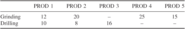
The factory has three grinding machines and two drilling machines and works a six-day week with two shifts of 8 hours on each day. Eight workers are employed in assembly, each working one shift a day.
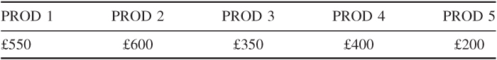
The problem is to find how much of each product is to be manufactured so as to maximize the total profit contribution.
This is a very simple example of the so-called ‘product mix’ application of LP.
In order to create a mathematical model, we introduce variables x1, x2, …, x5 representing the numbers of PROD 1, PROD 2, …, PROD 5 that should be produced in a week. As each unit of PROD 1 yields £550 contribution to profit and each unit of PROD 2 yields £600 contribution to profit, etc., our total profit contribution will be represented by the expression:
The objective of the factory is to choose x1, x2, …, x5 so as to make the value of this expression as high as possible, that is, Expression (1.1) is the objective function that we wish to maximize (in this case).
Clearly, our processing and labour capacities, to some extent, limit the values that the xj can take. Given that we have only three grinding machines working for a total of 96 hours a week each, we have 288 hours of grinding capacity available. Each unit of PROD 1 uses 12 hours grinding. x1 units will therefore use 12x1 hours. Similarly, x2 units of PROD 2 will use 20x2 hours. The total amount of grinding capacity that we use in a week is given by the expression on the left-hand side of Inequality (1.2):
Inequality (1.2) is a mathematical way of saying that we cannot use up more than the 288 hours of grinding available per week. Inequality (1.2) is known as a constraint. It restricts (or constrains) the possible values that the variables xj can take.
The drilling capacity is 192 hours a week. This gives rise to the following constraint:
1.3 ![]()
Finally, the fact that we have only a total of eight assembly workers each working 48 hours a week gives us a labour capacity of 384 hours. As each unit of each product uses 20 hours of this capacity, we have the constraint
We have now expressed our original practical problem as a mathematical model. The particular form that this model takes is that of an LP model. This model is now a well-defined mathematical problem. We wish to find values for the variables x1, x2, …, x5 that make expression (1.1) (the objective function) as large as possible but still satisfy constraints (1.2)–(1.4). You should be aware of why the term ‘linear’ is applied to this particular type of problem. Expression (1.1) and the left-hand sides of constraints (1.2)–(1.4) are all linear. Nowhere do we get terms like ![]() , x1x2 or log x appearing.
, x1x2 or log x appearing.
There are a number of implicit assumptions in this model that we should be aware of. Firstly, we must obviously assume that the variables x1, x2, …, x5 are not allowed to be negative, that is, we do not make negative quantities of any product. We might explicitly state these conditions by the extra constraints
In most LP models the non-negativity constraints (1.5) are implicitly assumed to apply unless we state otherwise. Secondly, we have assumed that the variables x1, x2, …, x5 can take fractional values, for example, it is meaningful to make 2.36 units of PROD 1. This assumption may or may not be entirely warranted. If, for example, PROD 1 represented gallons of beer, fractional quantities would be acceptable. On the other hand, if it represented numbers of motor cars, it would not be meaningful. In practice, the assumption that the variables can be fractional is perfectly acceptable in this type of model, if the errors involved in rounding to the nearest integer are not great. If this is not the case, we have to resort to IP.
The model above illustrates some of the essential features of an LP model:
Practical models will, of course, be much bigger (more variables and constraints) and more complicated but they must always have the above three essential features. The optimal solution to the above model is included in Section 6.2.
In order to give a wider picture of how LP models can arise, we give a second small example of a practical problem.
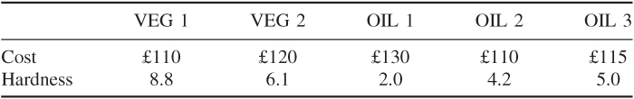
| Vegetable oils | VEG 1 VEG 2 |
| Non-vegetable oils | OIL 1 OIL 2 OIL 3 |
How should the food manufacturer make their product in order to maximize their net profit?
This is another very common type of application of LP although, of course, practical problems will be, generally, much bigger.
Variables are introduced to represent the unknown quantities. x1, x2, …, x5 represent the quantities (tons) of VEG 1, VEG 2, OIL 1, OIL 2 and OIL 3 that should be bought, refined and blended in a month. y represents the quantity of the product that should be made. Our objective is to maximize the net profit:
The refining capacities give the following two constraints:
1.8 ![]()
The hardness limitations on the final product are imposed by the following two constraints:
1.9 ![]()
1.10 ![]()
Finally it is necessary to make sure that the weight of the final product is equal to the weight of the ingredients. This is done by a continuity constraint:
The objective function (1.6) (to be maximized) together with constraints (1.7–(1.11) make up our LP model.
The linearity assumption of LP is not always warranted in a practical problem, although it makes any model computationally much easier to solve. When we have to incorporate non-linear terms in a model (either in the objective function or the constraints) we obtain an non-linear programming (NLP) model. In Chapter 7, we will see how such models may arise and a method of modelling a wide class of such problems using separable programming. Nevertheless, such models are usually far more difficult to solve.
Finally, the assumption that variables can be allowed to take fractional values is not always warranted. When we insist that some or all of the variables in an LP model must take integer (whole number) values we obtain an integer programming (IP) model. Such models are again much more difficult to solve than conventional LP models. We will see in Chapters 8–10 that IP opens up the possibility of modelling a surprisingly wide range of practical problems.
Another type of model that we discuss in Section 4.2 is known as a stochastic programming model. This arises when some of the data are uncertain but can be specified by a probability distribution. Although data in many LP models may be uncertain, their representation by expected values alone may not be sufficient. Situations in which a more explicit recognition of the probabilistic nature of data may be made, but the resultant model still converted to a linear program, are described. In Chapter 3, we mention chance-constrained models and in Chapter 4, multi-staged models with recourse, both of which fall in the category of stochastic programming. An example of the use of this latter type of model is given in Sections 12.24, 13.24 and 14.24 where it is applied to determining the price of airline tickets over successive periods in the face of uncertain demand. A good reference to stochastic programming is Kall and Wallace (1994).