Chapter 3

Building linear programming models

3.1 The importance of linearity

It was pointed out in Section 1.2 that a linear programming model demands that the objective function and constraints involve linear expressions. Nowhere can we have terms such as appearing. For many practical problems, this is a considerable limitation and rules out the use of linear programming. Non-linear expressions can, however, sometimes be converted into a suitable linear form. The reason why linear programming models are given so much attention in comparison with non-linear programming models is that they are much easier to solve. Care should also be taken, however, to make sure that a linear programming model is only fitted to situations where it represents a valid model or justified approximation. It is easy to be influenced by the comparative ease with which linear programming models can be solved compared with non-linear ones.

It is worth giving an indication of why linear programming models can be solved more easily than non-linear ones. In order to do this, we use a two-variable model, as it can be represented geometrically.

The values of the variables x₁ and x₂ can be regarded as the coordinates of the points in Figure 3.1.

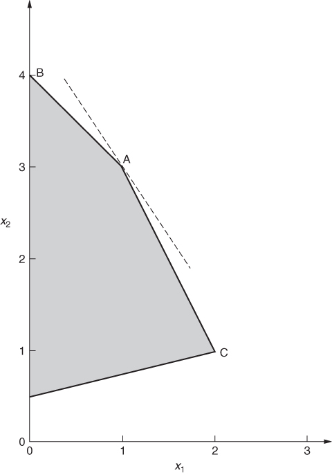
The optimal solution is represented by point A where 3x₁ + 2x₂ has a value of 9. Any point on the broken line in Figure 3.1 will give the objective 3x₁ + 2x₂ this value.

Other values of the objective correspond to a line parallel to this. It should be obvious geometrically that in any two-variable example, the optimal solution will always lie on the boundary of the feasible (shaded) region. Usually, it will occur at a vertex such as A. It is possible, however, that the objective lines might be parallel to one of the sides of the feasible region. For example, if the objective function in the above example were 4x₁ + 2x₂, the objective lines would be parallel to AC in Figure 3.1. The point A would then still be an optimal solution but C would be also, and any point between A and C. We would have a case of alternative solutions. This topic is discussed at greater detail in Sections 6.2 and 6.3. Our focus here, however, is to show that the optimal solution (if there is one) always lies on the boundary of the feasible region. In fact, even if the case of alternative solutions does arise, there will always be an optimal solution that lies at a vertex. This last fact generalizes to problems with more variables (which would need more dimensions to be represented geometrically). It is this fact that makes linear programming models comparatively easy to solve. The simplex algorithm works by only examining vertex solutions (rather than the generally infinite set of feasible solutions).

It should be possible to appreciate that this simple property of linear programming models may not apply well to non-linear programming models. For models with a non-linear objective function, the objective lines in two dimensions would no longer be straight lines. If there were non-linearities in the constraints, the feasible region might not be bounded by straight lines either. In these circumstances, the optimal solution might well not lie at a vertex. It might even lie in the interior of the feasible region. Moreover, having found a solution, it may be rather difficult to be sure that it is optimal (so-called local optima may exist). All these considerations are described in Chapter 7. Our purpose here is simply to indicate the large extent to which linearity makes mathematical programming models easier to solve.

Finally, it should not be suggested that a linear programming model always represents an approximation to a non-linear situation. There are many practical situations where a linear programming model is a totally respectable representation.

3.2 Defining objectives

With a given set of constraints, different objectives will probably lead to different optimal solutions. Nevertheless, it should not automatically be assumed that this will always happen. It is possible that two different objectives can lead to the same operating pattern. As an extreme case of this, it can happen that the objective is irrelevant. The constraints of a problem may define a unique solution. For example, consider the following three constraints:

3.1

3.2

3.3

These force the solution x₁ = x₂ = 1 no matter what the objective is. Practical situations do arise where there is no freedom of action and only one feasible solution is possible. If the model for such a situation is at all complicated, this property may not be apparent. Should different objective functions always yield the same optimal solution the property may be suspected and should be investigated as a greater understanding of what is being modelled must surely result. In fact, such a discovery would result in there being no further need for linear programming.

We now assume, however, that we have a problem, where the definition of a suitable objective is of genuine importance. Possible objectives that might be suggested for optimization by an organization are as follows:

Many other objectives could be suggested. It could well be that there is no desire to optimize anything at all. Frequently, a number of objectives will apply simultaneously. Possibly, some of these objectives will conflict. It is, however, our contention that mathematical programming can be relevant in any of these situations, that is, in the case of optimizing single objectives, multiple and conflicting objectives or problems where there is no optimization of the objective.

3.2.1 Single objectives

Most practical mathematical programming models used in operational research involve either maximizing profit or minimizing cost. The ‘profit’ that is maximized would usually be more accurately referred to as contribution to profit or the cost as variable cost. In a cost minimization, the cost incorporated in an objective function would normally only be a variable cost. For example, suppose each unit of a product produced cost £C. It would only be valid to assume that x units would cost £Cx if C were a marginal cost, that is, the extra cost incurred for each extra unit produced. It would normally be incorrect to add in fixed costs such as administration or capital costs of equipment. An exception to this does arise with some integer programming models when we allow the model itself to decide whether or not a certain fixed cost should be incurred; for example, if we do not make anything we incur no fixed cost, but if we make anything at all we do incur such a cost. Normally, however, with standard linear programming models, we are interested only in variable costs. Indeed, a common mistake in building a model is to use average costs rather than marginal costs. Similarly, when profit coefficients are calculated, it is only normally correct to subtract variable costs from incomes. As a result of this, the term profit contribution might be more suitable.

In the common situation where a linear programming model is being used to allocate productive capacity in some sort of optimal manner, there is often a choice to be made over whether simply to minimize cost or maximize profit. Normally, a cost minimization involves allocating productive capacity to meet some specified known demand at minimum cost. Such models will probably contain constraints such as

3.4

or something analogous, where x_ij is the quantity of product i produced by process j and D_i is the demand for product i.

Should such constraints be left out inadvertently, as sometimes happens, the minimum cost solution will often turn out to produce nothing! On the other hand, if a profit maximization model is built, it allows one to be more ambitious. Instead of specifying constant demands D_i, it is possible to allow the model to determine optimal production levels for each product. The quantities D_i would then become variables d_i representing these production levels. Constraints (3.4) would become

3.5

In order that the model can determine optimal values for the variable d_i, they must be given suitable unit profit contribution coefficients P_i in the objective function. The model would then be able to weigh up the profits resulting from different production plans in comparison with the costs incurred and determine the optimal level of operations. Clearly, such a model is doing rather more than the simpler cost minimization model. In practice, it may be better to start with a cost minimization model and get it accepted as a planning tool before extending the model to be one of profit maximization.

In a profit maximization model, the unit profit contribution figure P_i may itself depend on the value of the variable d_i. The term P_id_i in the objective function would no longer be linear. If P_i could be expressed as a function of d_i, a non-linear model could be constructed. An example of this idea is described by McDonald et al. (1974) in a resource allocation model for the health service.

A complication may arise in defining a monetary objective when the model represents activities taking place over a period of time. Some method has to be found for valuing profits or costs in the future in comparison with the present. The most usual technique is to discount future money at some rate of interest. Objective coefficients corresponding to the future will then be suitably reduced. Models where this might be relevant are discussed in Section 4.1 and are known as multiperiod or dynamic models. A number of problems presented in Part II give rise to such models. A further complication is illustrated by the ECONOMIC PLANNING problem of Part II. Here, decisions have to be made regarding whether or not to forego profit now in order to invest in new plant so as to make larger profits in the future. The relative desirabilities of different growth patterns lead to alternative objective functions.

3.2.2 Multiple and conflicting objectives

A mathematical programming model involves a single objective function that is to be maximized or minimized. This does not, however, imply that problems with multiple objectives cannot be tackled. Various modelling techniques and solution strategies can be applied to such problems.

A first approach to a problem with multiple objectives is to solve the model a number of times with each objective in turn. The comparison of the different results may suggest a satisfactory solution to the problem or indicate further investigations. A fairly obvious example of two objectives, each of which can be optimized in turn, is given by the MANPOWER PLANNING problem of Part II. Here, either cost or redundancy can be minimized. The computational task of using different objectives in turn is eased if each solution is used as a starting solution to a run with a new objective as mentioned in Section 2.3.

Objectives and constraints can often be interchanged, for example, we may wish to pursue some desirable social objective so long as costs do not exceed a specified level, or alternatively, we may wish to minimize cost using the social consideration as a constraint on our operations. This interplay between objectives and constraints is a feature of many mathematical programming models, which is far too rarely recognized. Once a model has been built, it is extremely easy to convert an objective into a constraint or vice versa. The proper use for such a model is to solve it a number of times, making such changes. An examination and discussion of the resultant solutions should lead to an understanding of the operating options available in the practical situation, which has been modelled. We therefore have one method of coping with multiple objectives through treating all but one objective as a constraint. Experiments can then be carried out by varying the objective to be optimized and the right-hand side values of the objective/constraints.

Another way of tackling multiple objectives is to take a suitable linear combination of all the objective functions and optimize that. It is clearly necessary to attach relative weightings or utilities to the different objectives. What these weightings should be may often be a matter of personal judgment. Again, it will probably be necessary to experiment with different such composite objectives in order to ‘map out’ a series of possible solutions. Such solutions can then be presented to the decision makers as policy options. Most commercial packages allow the user to define and vary the weightings of composite objective functions very easily. It should not be thought that this approach to multiple objectives is completely distinct from the approach of treating all but one of the objectives as a constraint. When a linear programming model is solved, each constraint has associated with it a ‘value’ known as a shadow price. These values have considerable economic importance and are discussed at length in Section 6.2. If these shadow prices were to be used as the weightings to be given to the objectives/constraints in the composite approach that we have described in this section, then the same optimal solution could be obtained.

When objectives are in conflict, as multiple objectives frequently will be to some extent, any of the above approaches can be adopted. Care must be taken, however, when objectives are replaced by constraints not to model conflicting constraints as such. The resultant model would clearly be infeasible. Conflicting constraints necessitate a relaxation in some or all of these constraints. Constraints become goals, which may, or may not, be achieved. The degree of over, or under, achievement is represented in the objective function. This way of allowing the model itself to determine how to allow a certain degree of relaxation is described in Section 3.3 and is sometimes known as goal programming.

There is no one obvious way of dealing with multiple objectives through mathematical programming. Some or all of the above approaches should be used in particular circumstances. Given a situation with multiple objectives in which there are no clearly defined weightings for the objectives no cut-and-dried approach can ever be possible. Rather than being a cause for regret, this is a healthy situation. It would be desirable if alternative approaches were adopted more often in the case of single objective models rather than a once only solution being obtained and implemented.

3.2.3 Minimax objectives

The following type of objective arises in some situations:

This can be converted into a conventional linear programming form by introducing a variable z to represent the above objective. In addition to the original constraints, we express the transformed model as

The new constraints guarantee that z will be greater than or equal to each of ∑ _ja_ijx_j for all i. By minimizing z, it will be driven down to the maximum of these expressions.

A special example of this type of formulation arises in goal programming and is discussed in Section 3.3.

It also arises in the formulation of zero-sum games as linear programmes.

Of course, a maximin objective can easily be dealt with similarly. It should, however, be pointed out that a maximax (or minimin) objective cannot be dealt with by linear programming and requires integer programming. This is discussed in Section 9.4.

3.2.4 Ratio objectives

In some applications, the following non-linear objective arises:

Rather surprisingly, the resultant model can be converted into a linear programming form by the following transformations.

It must be pointed out that this transformation is only valid if the denominator ∑ _jb_jx_j is always of the same sign and non-zero. If necessary (and it is valid), an extra constraint must be introduced to ensure this. If ∑ _jb_jx_j always be negative the directions of the inequalities in the constraints above must, of course, be reversed.

Once the transformed model is solved, the values of the x_j variables can be found by dividing w_j by t.

An interesting application involving this type of objective arises in devising performance measures for certain organizations where, for example, there is no profit criterion that can be used. This is described by Charnes et al. (1978). The objective arises as a ratio of weighted inputs and outputs of the organization variables represent the weighting factors. Each organization is allowed to choose the weighting factors so as to maximize its performance ratio subject to certain constraints. This subject is now known as data envelopment analysis (DEA). An illustration and description of its use are given by the EFFICIENCY ANALYSIS problem in Part II.

3.2.5 Non-existent and non-optimizable objectives

The phrase ‘non-optimizable objectives’ might be regarded as self-contradictory. We will, however, take the word ‘objective’, in this phrase, in the non-technical sense. In many practical situations, there is no wish to optimize anything. Even if an organization has certain objectives (such as survival), there may be no question of optimizing them or possibly any meaning to be attached to the word ‘optimization’ when so applied. Mathematical programming is sometimes dismissed rather peremptorily as being concerned with optimization when many practical problems involve no optimization. Such a dismissal of the technique is premature. If the problem involves constraints, finding a solution that satisfies the constraints may be by no means straightforward. Solving a mathematical programming model of the situation with an arbitrary objective function will at least enable one to find a feasible solution if it exists, that is, a solution that satisfies the constraints. The last remark is often very relevant to certain integer programming models, where a very complex set of constraints may exist. It is, however, sometimes relevant to the constraints of a conventional linear programming model. The use of a (contrived) objective is also of value beyond simply enabling one to create a well-defined mathematical programming model. By optimizing an objective, or a series of objectives, in turn, ‘extreme’ solutions satisfying the constraints are obtained. These extreme solutions can be of great value in indicating the accuracy or otherwise of the model. Should any of these solutions be unacceptable from a practical point of view, then the model is incorrect and should be modified if possible. As stated before, the validation of a model in this way is often as valuable, if not more valuable, an activity as that of obtaining solutions to be used in decision making.

3.3 Defining constraints

Some of the most common types of constraint that arise in linear programming models are classified below.

3.3.1 Productive capacity constraints

These are the sorts of constraints that arose in the product mix example of Section 1.2. If resources to be used in a productive operation are in limited supply, then the relationship between this supply and the possible uses made of it by the different activities give rise to such a constraint. The resources to be considered could be processing capacity or manpower.

3.3.2 Raw material availabilities

If certain activities (such as producing products) make use of raw materials that are in limited supply, then this clearly should result in constraints.

3.3.3 Marketing demands and limitations

If there is a limitation on the amount of a product that can be sold, which could well result in less of the product being manufactured than would be allowed by the other constraints, this should be modelled. Such constraints may be of the form

3.6

where x is the variable representing the quantity to be made and M is the market limitation.

Minimum marketing limitations might also be imposed if it were necessary to make at least a certain amount of a product to satisfy some demand. Such constraints would be of the form:

3.7

Sometimes Inequalities (3.6) or (3.7) might be ‘=’ constraints instead if some demand had to be met exactly.

The constraints (3.6) and (3.7) (or as equalities) are especially simple. When the simplex algorithm is used to solve a model, such constraints are more efficiently dealt with as simple bounds on a variable. This is discussed later in this chapter.

3.3.4 Material balance (continuity) constraints

It is often necessary to represent the fact that the sum total of the quantities going into some process equals the sum total coming out. For example, in the blending problem of Section 1.2, we had to ensure that the weight of the final product was equal to the total weight of the ingredients. Such conditions are often easily overlooked. Material balance constraints such as this will usually be of the form:

3.8

showing that the total quantity (weight or volume) represented by the x_j variables must be the same as the total quantity represented by the y_k variables. Sometimes, some coefficients in such a constraint will not be unity, but some value representing a loss or gain of weight or volume in a particular process.

3.3.5 Quality stipulations

These constraints usually arise in blending problems where certain ingredients have certain measurable qualities associated with them. If it is necessary that the products of blending have qualities within certain limits, then constraints will result. The blending example of Section 1.2 gave an example of this. Such constraints may involve, for example, quantities of nutrients in foods, octane values for petrols and strengths of materials.

We now turn our attention to a number of more abstract considerations concerning constraints that we feel a model builder should be aware of.

3.3.6 Hard and soft constraints

A linear programming constraint such as

3.9

obviously rules out any solutions in which the sum over j exceeds the quantity b. There are some situations where this is unrealistic. For example, if Inequality (3.9) represented a productive capacity limitation or a raw material availability, there might be practical circumstances in which this limitation would be overruled. It might sometimes be worthwhile or necessary to buy in extra capacity or raw materials at a high price. In such circumstances, (3.9) would be an unrealistic representation of the situation. Other circumstances exist in which it might be impossible to violate (3.9). For example, (3.9) might be a technological constraint imposed by the capacity of a pipe whose cross section could not be expanded. Constraints such as (3.9), which cannot be violated, are sometimes known as hard constraints. It is often argued that what we need are soft constraints that can be violated at a certain cost. If (3.9) were to be rewritten as

3.10

and u were given a suitable positive (negative) cost coefficient c for a minimization (maximization) problem, we would have achieved our desired effect. The variable b would represent a capacity or raw material availability that could be expanded to b + u at a cost cu if the optimization of the model found this to be desirable. Possibly the ‘surplus’ variable u would be given a simple upper bound as well to prevent the increase exceeding a specified amount.

If Inequality (3.9) were a ‘≥’ constraint, an analogous effect could be achieved by a ‘slack’ variable. If Inequality (3.9) be an equality constraint, it would be possible to allow the right-hand side coefficient b to be overreached or underreached by modelling it as

3.11

and giving u and v appropriately weighted coefficients in the objective function. It should be apparent that either u or v must be zero in the optimal solution. Any solution in which u and v came out positive could be adjusted to produce a better solution by subtracting the smaller of u and v from both of them.

An alternative way of viewing such soft constraints is through fuzzy sets, where a degree of membership corresponds to the amount by which the constraint is violated. It has, however, been shown by Dyson (1980) that formulations in terms of fuzzy set theory can be reformulated as conventional LP models with minimax objectives.

3.3.7 Chance constraints

In some applications, it is desired to specify that a certain constraint be satisfied with a given probability; for example, we may wish to be 95% confident that a constraint holds. This situation is written as

3.12

where β is a probability. In practice, one might expect larger values of β to correspond to higher costs, which should be reflected in the objective function. This would create a more complicated model. Should no relationship between the value of β and the cost be known (as is often the case) then a rather crude, but sometimes satisfactory, approach is to replace Inequality (3.12) by a deterministic equivalent. We would then replace (3.12) by

3.13

where b′ is a number larger than b such that the satisfaction of (3.13) implies Inequality (3.12). This idea is due to Charnes and Cooper (1959).

3.3.8 Conflicting constraints

It sometimes happens that a problem involves a number of constraints, not all of which can be satisfied simultaneously. A conventional model would obviously be infeasible. The objective in such a case is sometimes stipulated to be to satisfy all the constraints as nearly as possible. We have the case of conflicting objectives referred to in Section 3.2 but postponed to this section.

The type of model that this situation gives rise to is sometimes known as a goal programming model. This term was invented by Charnes and Cooper (1961b), but the type of model that results is still a linear programming model.

Each constraint is regarded as a ‘goal’ that must be satisfied as nearly as possible. For example, if we wished to impose the following constraints:

3.14

but wanted to allow the possibility of them not all being satisfied exactly, we would replace them by the ‘soft’ constraints

3.15

We are clearly using the same device described before.

Our objective would be to make sure that each such constraint (3.14) is as nearly satisfied as possible. There are a number of alternative ways of making such an objective specific. Two possibilities are as follows:

For many practical problems which of the above objectives is used is not very important.

Objective 1 can be dealt with by defining an objective function consisting of the sum of the slack (u) and surplus (v) variables in the constraints such as Equation (3.15). Possibly, these variables might be weighted in the objective with non-unit coefficients to reflect the relative importance of different constraints. An example of the use of such an objective is given in the MARKET SHARING problem of Part II. The fact that this is an integer programming model does not affect the argument, as such models could equally well result from linear programming models. A linear programming application arises in the CURVE FITTING problem.

Objective 2 is slightly more complicated to deal with but can surprisingly still be accomplished in a linear programming model. An extra variable z is introduced. This variable represents the maximum deviation. We, therefore, have to impose extra constraints.

3.16

3.17

The objective function to be minimized is simply the variable z. Clearly, the optimal value of z will be no greater than the maximum of u_i and v_i by virtue of optimality. Nor can it be smaller than any of u_i or v_i by virtue of the constraints (3.16) and (3.17). Therefore, the optimal value of z will be both as small as possible and exactly equal to the maximum deviation of ∑ _ja_ijx_j from its corresponding right-hand side b_i. This type of problem is sometimes known as a bottleneck problem. Both the CURVE FITTING and MARKET SHARING problems illustrate this type of objective.

An interesting example of such a minimax objective is described by Redpath and Wright (1981) in an application of linear programming to deciding levels and directions for irradiating cancerous tumours. As an alternative to minimizing the variance of radiation across a tumour, they minimize the maximum difference of radiation levels. This can clearly be done by computationally easier linear programming rather than quadratic programming.

Hooker and Williams (2012) show how equity, in the form of a minimax objective, can be combined with a utilitarian objective in an integer programming model.

3.3.9 Redundant constraints

Suppose we have a constraint such as

3.18

in a linear programming model. If, in the optimal solution, the quantity ∑ _ja_jx_j turns out to be less than b, then the constraint (3.18) will be said to be non-binding (and have a zero shadow price). Such a non-binding constraint could just as well be left out of the model, as this would not affect the optimal solution. There may well, however, be good reasons for including such redundant constraints in a model. First, the redundancy may not be apparent until the model is solved. The constraint must, therefore, be included in case it turns out to be binding. Second, if a model is to be used regularly with changes in the data, then the constraint might become binding with some future data. There would then be virtue in keeping the constraint to avoid a future remodelling. Third, ranging information, which is discussed in Section 6.3, depends on constraints that may well be redundant in the sense of not affecting the optimal solution.

It should be noted that a constraint such as (3.18) can be non-binding even if the quantity ∑ _ja_jx_j is equal to b. This happens if the removal of the constraint does not affect the optimal solution, that is, ∑ _ja_jx_j must be equal to b for reasons other than the existence of constraint (3.18). Such non-binding constraints are recognized by there being a zero shadow price on the constraint in the optimal solution. Shadow prices are discussed in Section 6.2.

For ‘≥’ constraints, analogous results hold. If Inequality (3.18) were such a constraint, it would be non-binding if ∑ _ja_jx_j exceeded b but possibly still non-binding if ∑ _ja_jx_j equalled b.

Finally, it should be pointed out that with integer programming, it would not be true to say that if ∑ _ja_jx_j were less than b in Inequality (3.18) then Inequality (3.18) would be non-binding. Inequality (3.18) could well be binding and, therefore, not redundant. This is discussed in Section 10.3.

The advisability or otherwise of including redundant constraints in a model is discussed in Section 3.3. A quick method of detecting some such redundancies is also described.

3.3.10 Simple and generalized upper bounds

It was pointed out that marketing constraints often take the particularly simple forms of Inequality (3.6) or (3.7). Simple bounds on a variable such as these are more efficiently dealt with through a modification of the simplex algorithm. Most commercial package programmes use this modification. Such bounds are not, therefore, specified as conventional constraints but specified as simple bounds for the appropriate variables. A generalization of simple bounds known as generalized upper bounds (GUBs) also proves to be of great computational value in solving a model and therefore worth recognizing. Such constraints are usually written as

3.19

The set of variables x_j is said to have a GUB of b. This means that the sum of these variables must be b. If Equation (3.19) were a ‘≤’ constraint instead of an equality, the addition of a slack variable would obviously convert it to the form (Equation 3.19). The fact that the coefficients of the variables in Equation (3.19) are unity is not very important, as scaling can always convert any constraint with all non-negative coefficients into this form. What is, however, important is that when a number of constraints such as Equation (3.19) exist, the variables in them form exclusive sets. A set of variables is said to belong to the GUB set, if it can belong to no others. If variables are specified as belonging to GUB sets, it is not necessary to specify the corresponding constraints such as Equation (3.19). A further modification of the simplex algorithm copes with the implied constraint in an analogous way to simple bounding constraints. The diagrammatic representation of a model in Figure 3.2 shows three GUB-type constraints. These constraints could be removed from the model and treated as GUB sets.

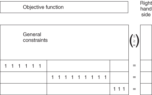
There is normally only virtue in using the GUB modification of the simplex algorithm if a large number of GUB sets can be isolated. For example, in the transportation problem, which is discussed in Section 5.3, it can be seen that at least half of the constraints can be regarded as GUB sets.

The computational advantages of recognizing GUB constraints can be very great indeed with large models. A way of detecting a large number of such sets if they exist in a model is described by Brearley et al. (1975).

3.3.11 Unusual constraints

In previous sections, we have concentrated on constraints that can be modelled using linear programming. It is important, however, not to dismiss ‘unusual’ restrictions that may arise in a practical problem as not being able to be so modelled. By extending a model to be an integer programming model, it is sometimes possible to model such restrictions. For example, a restriction such as

We can only produce product 1 if product 2 is produced but neither of products 3 or 4 are produced.

could be modelled. This topic is discussed much further in Chapter 9.

3.4 How to build a good model

Possible aims that a model builder has when constructing a model are the ease of understanding the model, detecting errors in the model and computing the solution. Ways of trying to achieve and resolve these aims are described below.

3.4.1 Ease of understanding the model

It is often possible to build a compact but realistic model when quantities appear implicitly rather than explicitly, for example, instead of a non-negative quantity being represented by a variable y and being equated to an expression f(x) by the constraint

3.20

the variable y does not appear, but f(x) is substituted into all the expressions where it would appear. Building such compact models often leads to great difficulty and extra calculation in interpreting the solution. Even though a less-compact model takes longer to solve, it is often worth the extra time. If, however, a report writer is used, this may take care of interpretation difficulties, and the use of compact models is desirable from the point of view of the third aim.

It is also desirable to use mnemonic names for the variables and constraints in a problem to ease the interpretation of the solution. The computer input to the small blending problem illustrated in Section 1.2 shows how such names can be constructed. A very systematic approach to naming variables and constraints in a model is described by Beale et al. (1974).

3.4.2 Ease of detecting errors in the model

This aim is clearly linked to the first. Errors can be of two types: (i) clerical errors such as bad typing and (ii) formulation errors. To avoid the first type of error, it is desirable to build any but very small models using a matrix generator (MG) or language.

There is also great value to be obtained from using a PRESOLVE or REDUCE procedure on a model for error detection. Clerical or formulation errors often result in a model being unbounded or infeasible. Such conditions can often be revealed easily using such a procedure. A simple procedure of this kind, which also simplifies models, is outlined below.

Formulation can sometimes be done with error detection in mind. This point is illustrated in Section 6.1.

3.4.3 Ease of computing the solution

LP models can use large amounts of computer time, and it is desirable to build models that can be solved as quickly as possible. This objective can conflict with the first. In order to meet the first objective, it is desirable to avoid compact models. If a PRESOLVE or REDUCE procedure is applied after the model has been built, but before solving it, then dramatic reductions in size can sometimes be achieved. An algorithm for doing this is described by Brearley et al. (1975). Karwan et al. (1983) provided a collection of methods for detecting redundancy. The reduced problem can then be solved, and this solution used to generate a solution to the original problem.

In order to illustrate the possibility of spotting redundancies in a linear programming model, we consider the following numerical example:

3.21

3.22

3.23

3.24

3.25

As x₃ has a negative objective coefficient and the problem is one of maximization, it is desirable to make x₃ as small as possible, x₃ has positive coefficients in constraints (3.22) and (3.23). As these constraints are both of the ‘≤’ type, there can be no restriction on making x₃ as small as possible. Therefore, x₃ can be reduced to its lower bound of zero and hence be regarded as a redundant variable.

Having removed the variable x₃ from the model, constraint (3.23) is worthy of examination. All the coefficients in this constraint are now negative. Therefore, the value of the expression on the left-hand side of the inequality relation can never be positive. This expression must, therefore, always be smaller than the right-hand side value of 1, indicating that the constraint is redundant and may be removed from the problem.

The above model could, therefore, be reduced in size. With large models, such reductions could well lead to substantial reductions in the amount of computation needed to solve the model. Infeasibilities and unboundedness can also sometimes be revealed by such a procedure. A model is said to be infeasible, if there is no solution that satisfies all the constraints (including non-negativity conditions on the variables). If, on the other hand, there is no limit to the amount by which the objective function can be optimized, the model is said to be unbounded. Such conditions in a model usually suggest modelling errors and are discussed in detail in Section 6.1.

Some package programmes have procedures for reducing models in this way. Such procedures go under names such as REDUCE, PRESOLVE and ANALYSE. Problem reduction can be taken considerably further. Using simple bounds on variables and considering the dual model (the dual of a linear programming model is described in Section 6.2), the above example can be reduced to nothing (completely solved). A more complete treatment of reduction is beyond the scope of this book, as such reduction procedures are usually programmed and carried out automatically. It is not, therefore, always important that a model builder knows how to reduce his or her model, although the fact that it can be simply reduced must have implications for the situation being modelled. A much fuller treatment of the subject is given in Brearley et al. (1975) and Karwan et al. (1983).

Substantial reduction in computing time can also often be achieved by exploiting the special structure of a problem. One such structure that has proved particularly valuable is the GUB as described in Section 3.3. It is obviously desirable that the model builder detects such structure if it be present in a problem, although a few computer packages have facilities for doing this automatically through procedures such as those described by Brearley, Mitra and Williams.

3.4.4 Modal formulation

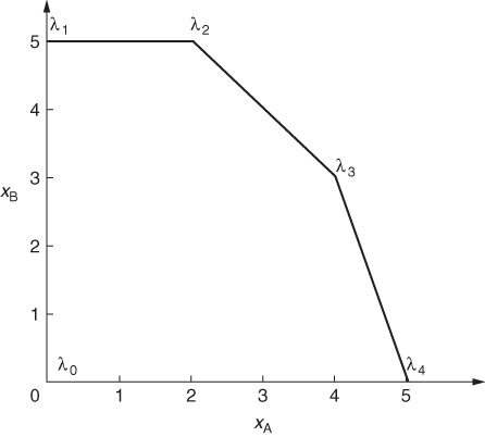
In large LP problems, reduction in the number of constraints can be achieved using modal formulations. If a series of constraints involves only a few variables, the feasible region for the space of these variables can be considered. For example, suppose that x_A and x_B are two of the (non-negative) variables in an LP model, and they occur in the following constraints:

3.26

3.27

3.28

The situation can be modelled, as demonstrated in Figure 3.3, by letting the activities for the ‘extreme modes’ of operation be represented by variables instead of x_A and x_B. If these variables are λ₀, λ₁, λ₂, λ₃ and λ₄, we only have to specify the single constraint.

3.29

Whenever x_A and x_B occur in other parts of the model, apart from constraints (3.26), (3.27) and (3.28) that are now ignored, we substitute the following expressions:

3.30

3.31

The coefficients for x_A are the ‘x_A coordinates’ of λ₁, λ₂, …, in Figure 3.3 and the coefficients of x_B are the ‘x_B coordinates’.

In this case, we have saved two constraints. The ingenious use of this idea can result in substantial savings in the number of constraints in a model.

Experiments in the use of a special case of this technique are described by Knolmayer (1982). Smith (1973) discusses the use of this approach to modelling practical problems. Modal formulations are quite common for particular processes in the petroleum industry. The REFINERY OPTIMIZATION model demonstrates a very simple case of this, where a process has only one mode of operation with inputs and outputs in fixed proportions. In this case, it is better to model the level of the process as an activity to avoid having to represent the (fixed) relationships between the inputs and outputs by constraints.

A general methodology for modelling processes with different types of input–output relations is developed by Müller-Merbach (1987).

3.4.5 Units of measurement

When a practical situation is modelled, it is important to pay attention to the units in which quantities are measured. Great disparity in the sizes of the coefficients in a linear programming model can make such a model difficult, if not impossible, to solve. For example, it would be stupid to measure profit in pounds if the unit profit coefficients in the objective function were of the order of millions of pounds. Similarly, if capacity constraints allowed quantities in thousands of tons, it would be better to allow each variable to represent a quantity in thousands of tons rather than in tons. Ideally, units should be chosen so that each non-zero coefficient in a linear programming model is of a magnitude between 0.1 and 10. In practice, this may not always be possible. Most commercial package programmes have procedures for automatically scaling the coefficients of a model before it is solved. The solution is then automatically unscaled before being printed out.

3.5 The use of modelling languages

A number of computer software aids exist for helping users to structure and input their problem into a package in the form of a model. Programmes to do this are sometimes known as matrix generators (MGs). Some such systems are more usefully thought of as special purpose high level programming languages and are, therefore, known as modelling languages.

It is now recognized that the main hurdle to the successful application of a mathematical programming model is often no longer the problem of computing the solution. Rather, it lies with the interface between the user and the computer. Some of the difficulties can be overcome by freeing the modeller from the specific needs of the package used to solve the model.

An ambitious attempt to overcome the user interface problems is described by Greenberg (1986). A survey of modelling systems is given by Greenberg and Murphy (1992).

Other systems are described by Buchanan and McKinnon (1987) and Greenberg et al. (1987). These systems pay attention to the output interface as well as the input.

A number of quite distinct approaches to building MGs/languages are described below. Before doing this, however, we specify the main advantages to be gained from using them.

3.5.1 A more natural input format

The input formats required by most packages are designed more with the package in mind than the user. As described in Section 2.2, most commercial packages use the MPS format. This orders the model by columns in a fixed format based on the internal ordering of the matrix in the computer. This is often unnatural, tedious, and a source of clerical error. In addition, this format is far from concise, requiring a separate data statement for every two coefficients in the model. The use of a modelling language can overcome all these disadvantages.

3.5.2 Debugging is made easier

As with computer programming, the debugging and verification of a model is an important and sometimes time-consuming task. The use of a format that the modeller finds natural makes this task much easier.

3.5.3 Modification is made easier

Models are often used on a regular basis with minor modifications, or once built may be used experimentally many times with small changes in data. The separation of the data (which changes) from the structure of the model, in most modelling languages, facilitates this task.

3.5.4 Repetition is automated

Large models usually arise from the combination or repetition of smaller models, for example, multiple periods, plants or products, as described in Section 4.1. In such circumstances, there will be a lot of repetition of particular items of data and structure. Formats such as MPS demand a repetition of this data, which is both inefficient and a potential source of error. Modelling languages generally take account of such repetition very easily through the indexing of time periods, etc.

Some of the distinct approaches adopted by different modelling languages are outlined below. Fourer (1983) also provides a very good and comprehensive discussion. The methods can only be understood in detail through the manuals of the relevant systems.

3.5.5 Special purpose generators using a high level language

It is possible to write a different program, in a general language, for each model one wishes to build. This approach ignores the similarities in structure that all mathematical programming models have, however diverse their application area, as well as the standard format required (e.g. MPS), which is tedious to remember and incorporate into a general program. It seems more sensible to incorporate such similarities into a language.

3.5.6 Matrix block building systems

The often huge matrix of coefficients in a practical model always exhibits a high degree of structure. The matrix tends to consist of small dense blocks of coefficients in an otherwise very sparse matrix. These blocks are often repetition of each other and are linked together by simple matrices such as identity matrices. The systematic combination and replication of submatrices into larger matrices in this way is the method used in certain systems. Such systems have functions that, for example, concatenate and transpose matrices. A defect of such systems is that they still require users to think in terms of matrices of coefficients, even though they free them from some of the mechanics of assembling such matrices.

3.5.7 Data structuring systems

Some systems allow the user to structure a model in a diagrammatic form. Flow diagrams are often particularly helpful. For example, a problem may involve flows of different raw materials into processes to give products that are then distributed via depots to customers. The system will allow the user to translate this representation into the system directly, avoiding algebraic notation. Such systems can be useful for specific applications, for example, process industries. They do have the defect that the user needs to learn quite a lot about the system before he or she can use it.

3.5.8 Mathematical languages

The above approaches all avoid the use of conventional notation, that is, ‘∑’ notation and indexed sets. Indeed, an argument sometimes used in their favour is that mathematical notation is unnatural to certain users who prefer to think of their model in other ways. This may well be the case with certain established applications (e.g. the petroleum industry), where mathematical programming is so established and important for a conceptual methodology of its own to have developed. If more generality is required, then conventional mathematical notation provides a language that is widely understood as well as providing a concise way of defining many models. The fact that the notation is so widely understood by anyone with an elementary mathematical training makes learning to use such a system comparatively easy.

Most general modelling systems, based on mathematical notation, are very similar. We describe their common features. We then illustrate this by a formulation of one of the models in Part II using a typical language NEWMAGIC. It is easy to translate such a model into any of the other, similar, modelling languages. Such languages require the user to identify the following components of their model. It is straightforward to see how these elements are used by means of the example below (although different systems will have varied key words and syntax rules).

3.5.8.1 SETs

These usually represent indices for certain classes of linear or integer programming variables. For example, PROD1, PROD2, PROD57 might be the variables representing 57 different products that vary only in their profits and resource usages. We could define a ‘root name’ PROD followed by an index from a SET A = {1, …, 57}. In most systems, indices can be numbers or names (e.g. towns or months of the year).

3.5.8.2 DATA

These are usually coefficients for the model, which may be defined in arrays or read from external files. The items in the arrays or files are often indexed by the indices described above.

3.5.8.3 VARIABLES

These are the linear or integer programming variables that appear in the model, typically defined using a root name together with associated indices, for example, PROD[A]. If the variable is of a special sort, for example, integer, free, binary, etc., this is usually specified with the variable.

3.5.8.4 OBJECTIVE

This is the Objective Function of the model given with MAXIMIZE or MINIMIZE. It is given a name and usually defined using ∑ notation over index sets defined above but by means of key words such as sum or sigma (as most keyboards do not support the symbol ∑).

3.5.8.5 CONSTRAINTS

These are the conventional linear constraints. They will, probably, also be indexed.

In addition, such languages will have many other facilities and features that are specific to the language and are not discussed in this chapter, but explained in the associated manuals. We give the example in NEWMAGIC below. As with other languages, it is convenient to include comments that are done here by including them between the symbols /*, or on a line preceded by !.

   MODEL FoodB
   DATA
      max t = 6, max i = 5;
   SET
      A = {1..2}, B = {1..5},
      T = {1..max t}, I = {1..max i};
   DATA
      cost[T,I] << " cost.dat ",
      hard[I] = [8,8,6.1,2.0,4.2,5.0];
   VARIABLES
      b[I,T], u[I,T], s[I,T], Prod[T];
   OBJECTIVE
   MAXIMIZE
      prof = sum{t in T} (150 * Prod[t] − sum{i in I} (cost[t,i] *
b[i,t] + 5 * s[i,t]));
   CONSTRAINTS
      loil{i in I, 1} : 500 + b[i,1] − u[i,1] − s[i,1] = 0,
      loil{i in I, t in T, t> 1} : s[i, t − 1] + b[i,t] − u[i,t]
− s[i,t] = 0,
      vveg{t in T} : sum{i in A} u[i,t] < = 200,
      voil{t in T} : sum{i in B} u[i,t] < = 250,
      lhrd{t in T} : 3 * Prod[t] < = sum{i in I} hard[i] * u[i,t],
      uhrd{t in T} : sum{i in I} hard[i] * u[i,t] < 6 * Prod[t],
      cont{t in T} : sum{i in I} u[i,t] = Prod[t],
   /* Specify bounds for the variables */
      for{i in I, t in T, t < maxt} s[i,t] < = 1000,
      for{i in I} s[i, maxt] = 500;
   /* This is the end of the continuous part of the model. The
   section below adds integer variables and extra constraints
   to model some logical conditions. Separate VARIABLE and
   CONSTRAINT sections are not necessary; they could be included
   in the VARIABLE and CONSTRAINT sections above. The keyword
   BINARY means an integer variable that can only take the
   values 0 or 1 */
   VARIABLES
   d[I,T] BINARY;
   CONSTRAINTS
   for{t in T}
   {
   ! Formulate second condition
   for{i in A}
   { ! UB on amount of veg. oil refined/month = 200
   20 * d[i,t] <= u[i,t], u[i,t] <= 200 * d[i,t]
   },
   for{i in B}
   {! UB on amount of non-veg. oil refined/month = 250
   20 * d[i,t] <= u[i,t], u[i,t] <= 250 * d[i,t]
   },
   ! Formulate first condition
   sum{i in I} d[i,t] <= 3,
   ! Formulate third condition
   d[1,t] <= d[5,t], d[2,t] <= d[5,t]
   };
   END MODEL
   SOLVE FoodB;
   PRINT SOLUTION FOR FoodB>> “FoodB.sol”;
   QUIT;