
Chapter 13
Active Sonar: Port/Starboard Discrimination
on Very Low Frequency Triplet Arrays1
13.1. Introduction
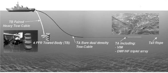
Very low frequency activated sonars have an operating wavelength close to 1 m and use towed arrays with acoustic lengths of several tens of meters. An example of such a system is displayed in Figure 13.1. In their conventional version, these arrays consist of one line of acoustic sensors (hydrophones) embedded in the center of an elastomer hose. They suffer a limitation due to the symmetry of revolution of the array: the output of a beam steered by compensating the delays of propagation in a given direction is the same on a cone (see Figure 13.3a) whose axis is the array axis. The maximum of the beam response, which indicates the direction of the target, is therefore a cone. For targets of interest, which are at long distances with respect to the depth of water, their direction is given by the intersection of the horizontal plane and the cone, which corresponds therefore to two symmetrical directions with respect to the array. The system cannot discriminate between port and starboard: this is the so-called “port-starboard ambiguity” problem. In active sonar, it is mandatory to solve this ambiguity at each sonar transmission (ping), as the alerted submarine may maneuver between two successive transmissions and may be detected only on one ping.
To solve this problem, one solution is to use two parallel arrays spaced one quarter of wavelength from each other. By recombining the signals of the two arrays, it is possible to discriminate between port and starboard. However, this solution has several drawbacks:
– Accurate control of the arrays geometry is not straightforward, and the knowledge of the accurate position of the hydrophones during navigation, in particular during maneuvers, requires specific instrumentation.
– Automatic deployment and recovery of the system from a ship at sea is difficult.
– The system is tuned in terms of frequency and is not easily extended to a wideband multi-octave sonar.
The solution discussed in this chapter relies on the concept of a triplet of hydrophones integrated in each section of the array; the number three accommodating for the roll of the towed array, which cannot be controlled during navigation. With the array section being of an order of 5 to 10 cm, the challenge is to combine port-starboard rejection and detection gain in a section that is 1/20th of the wavelength.
Figure 13.1. Overview of a very low frequency activated sonar system
13.2. Port/starboard beamforming on a triplet array
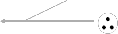
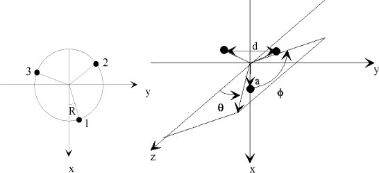
The geometry of the acoustic sensors of a triplet array is shown in Figure 13.2. The array is also fitted with roll sensors allowing us to permanently monitor its attitude and torsion, and whose outputs are fed in the beamforming algorithm. The shape of a beam formed on a single line towed array is shown in Figure 13.3a. It shows a symmetry of revolution. In order to solve the port/starboard (P/S) ambiguity, the ideal required beam response is shown in Figure 13.3b. Two beamforming techniques aiming at this objective are discussed below.
Figure 13.2. Triplet array geometry of acoustic sensors
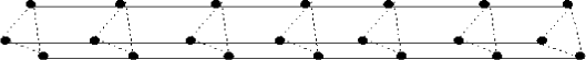
Figure 13.3a. Ambiguous beam on a monoline linear array
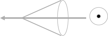
Figure 13.3b. Non ambiguous beams on a triplet array
13.2.1. Conventional (or cardioid) beamforming and limitations
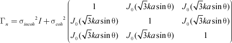
One way to solve the P/S ambiguity with several parallel line arrays consists, for each possible bearing of the target, of forming two beams: one port and one starboard, each with a null in the ambiguous direction. More precisely, let ![]() be the array manifold steering vector for one triplet of hydrophones associated with a plane wave from direction (θ,φ); its jth (j=0,1,2) component reads:
be the array manifold steering vector for one triplet of hydrophones associated with a plane wave from direction (θ,φ); its jth (j=0,1,2) component reads:
![]()
where:
θ is the bearing angle;
φ is the elevation angle, usually close to ±π/2;
λ is the wavelength;
k = 2π/λ;
a is the triplet radius;
R is the triplet roll;
j is the hydrophone number within a triplet: φj = 2jπ/3, j=0,1,2;
and where the angle definitions are given in Figure 13.4.
The cardioid steering vector ![]() (θ,φ) is obtained by imposing a null in the ambiguous direction. Its components for the steering direction (θ,φ+) read:
(θ,φ) is obtained by imposing a null in the ambiguous direction. Its components for the steering direction (θ,φ+) read:
![]()
where φ− = − φ+ corresponds to the ambiguous direction elevation. The beamforming output reads:
![]()
where the symbol (+) means complex conjugate and transpose, and where X(f) is the vector containing the triplet signals at frequency f.
This procedure is applied for bearing angles between 30° and 120°. Beyond, this the projection of the array section on the steering direction is too small and the beamforming is progressively modified towards a summation of the three arrays for 0° and 180°, in order to avoid too large signal losses, as detailed below.
Figure 13.4. Triplet geometry and frame of reference
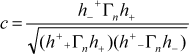
Triplet processing performances are fully characterized by the following quantities (see [DOI 95]):
a) The array gain G, in terms of signal-to-noise ratio, with respect to the monoline beamforming, which reads:
![]()
where Гn is the noise covariance matrix at the output of the monoline beamforming. For a mixture of uncorrelated and spherical isotropic noises, it can be shown that it reads:
where σ2 is the total noise power at monoline beamforming output: ![]() , and I the identity matrix. From the above expressions, we obtain (for a null roll angle):
, and I the identity matrix. From the above expressions, we obtain (for a null roll angle):
![]()
b) The port / starboard rejection ratio defined as:
![]()
This ratio is theoretically infinite, by construction, for the cardioid beamforming.
c) The noise correlation coefficient between port and starboard beams:
As can be seen from the expression of G, the main limitation of the cardioid beamforming arises from the fact that, for uncorrelated noise, the gain tends to zero when the value of k.a tends to zero: the constraint to form a null in the ambiguous direction leads to signal-to-noise losses when the transverse direction of the array is small with respect to the wavelength. Main sources of uncorrelated noise on a linear towed array are:
– electronic noise, which can be managed by a proper design of the electronic chain;
– flow noise, whose correlation coefficient within a triplet is small, because it is connected to the larger turbulence scale, which is the hose diameter.
Figure 13.5. Signal-to-noise gain of cardioid beamforming vs bearing – flow noise
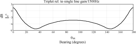
Values of the gain G, in dB, versus bearing, for a frequency of 1,500 Hz are shown in Figure 13.5. The external diameter of the array is 85 mm, and flow noise is dominant: it can be seen that the loss is 4 dB at broadside, and reaches 8 dB for bearings 30° and 120°. Beyond these values, cardioid processing is modified.
13.2.2. Adaptive port-starboard beamforming
The objective of the adaptive beamforming described in this section is to combine detection gain and P/S discrimination capability. Its design must take into account the structure of the target signal in activity, which has a limited time duration. Its impulse response duration can be estimated between 10 ms and 40 ms. This extension is related to the size of the target, and to the underwater propagation characteristics. To obtain good rejection capability, this signal must contribute significantly to the covariance matrix estimation. The matrix estimation time must therefore not be too large with respect to the echo duration, as would be the case if the estimation where performed directly on the many sensors of the full array. The processing described in this section is shown in Figure 13.6. The main steps are:
– conventional bearing beamforming independently on each of the monoline sub-arrays. The output signal of bearing beam m of array l (l=1 to 3) at time t reads:
![]()
– covariance marix (dimension 3×3) estimation obtained from the signals of the three beams steered at the same bearing on the three linear sub-arrays:
![]()
where the estimation is performed on a duration of an order of 20 ms;
– port-starboard beamforming. The output signal of the beam (+) for the bearing m reads:
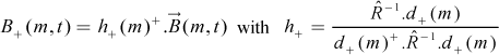
where d+(m) is the steering vector for bearing m and elevation φ+ associated with the phase center of the sub-arrays, as defined in the above section. A similar expression holds for direction (−) with d−(m).
The output energy is then determined on the same time interval as the one used for the covariance matrix estimation (Capon algorithm):
![]()
Notes:
– the available bandwidth B of the transmitted waveforms ranges typically from 500 Hz to 1,000 Hz, which corresponds to a number of independent snapshots for the covariance matrix estimation of N=10 to 20, for K=3 degrees of freedom;
– the phase centers of the sub-arrays are about 5 cm apart. This distance is much smaller than the range resolution (c/B ≈ 1.5 m), which allows us to use the narrowband approximation when implementing the processing;
– the detection loss related to the covariance matrix estimation over a finite number of independent snapsots can be assessed within the framework of the Van der Spek model [SPE 71], extended fluctuating target) invoking Capon’s theorem [CAP 70].
For a source of spectral density γs with bearing m and on side du ± (starboard or port) within noise described by the covariance matrix Гn, the total covariance matrix reads:
![]()
The effect of the adaptive beamfoming can be understood as follows:
– For the steering direction aimed at the target, a noise reference excluding the target is formed, and the corresponding signal is subtracted from the beam steered at the target, so that optimal detection performance is obtained in principle.
– For the steering direction aimed at the ambiguous direction, a noise reference containing the target signal is constructed, and the corresponding signal is subtracted from the beam steered at the ambiguous direction.
Target contribution is thus subtracted from the ambiguous direction, and P/S discrimination is thus obtained. The target signal is subtracted until its level become equal to the output noise. In the case of correlated noise, target rejection also provides signal-to-noise improvement, and the P/S rejection ratio is larger than the input signal-to-noise ratio (at monoline array output). In the case of uncorrelated noise, target rejection provides a signal-to-noise loss (signal loss effect due to the small size of the triplet w.r. to wavelength), and the P/S rejection ratio is smaller than the input signal-to-noise ratio (by an amount equal to G).
With this adaptive processing, optimal detection is obtained, regardless of the environmental conditions, while getting P/S rejection.
Figure 13.6. Adaptive port-starboard beamforming
Theoretical performances are obtained using the same quantities as in the previous section:
a) The signal-to-noise gain reads:
![]()
which leads to the following expression:
![]()
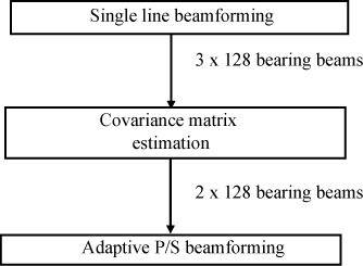
Values of the gain G, in dB, versus bearing, for a frequency of 1,500 Hz are shown in Figure 13.5. External diameter of the array is 85 mm, and flow noise is dominant, in the same conditions as in the previous section. It can be seen that the gain is always positive.
b) Expression for the P/S rejection ratio reads:
![]()
Values of r (in dB) versus bearing angle, at a frequency of 1,500 Hz and an array of external diameter 85 mm are shown in Figure 13.8, when flow noise is dominant, in the same conditions as in previous section. Input signal-to-noise ratio is also shown.
c) Noise correlation coefficient between starboard and port beams reads:
![]()
in the case of low input signal-to-noise ratio.
This last relation is quite remarkable and shows that the noise correlation coefficient between starboard and port beams is equal to the reciprocal of the P/S rejection, whatever the initial noise correlation.
The probability Pps to solve the port-starboard ambiguity in this case has been studied [DOI 95], where it has been shown that even very low values of the rejection (20 log r = 3 dB) enabled us to decide on which side the target is with Pps=0.99. This result arises from the fact that when the rejection ratio tends to 1, noise becomes fully correlated between the two hypotheses.
Figure 13.7. Signal-to-noise gain of adaptive beamforming vs bearing — flow noise
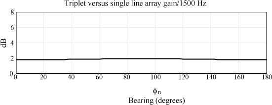
Figure 13.8. Port-starboard rejection ratio vs — flow noise
13.2.3. Experimental at-sea results
An experiment involving a very low frequency activated sonar and a cooperative target was conducted during the summer of 1999, in the Bay of Biscay, north of La Corogna. The sonar transmitted waveform was a hyperbolic frequency modulation type, at center frequency 1,500 Hz, with a 500 Hz bandwidth. Reception was performed on a triplet towed array.
The results of 60 successive sonar sweeps (“pings”) at the processing output are displayed in Figure 13.9 for the two beamforming described above: cardioid beamforming (left image) and adaptive beamforming (right image). The displays show the sweep number along the Oy axis versus the bearing angle (from 0 to 360°).
Figure 13.9. Cardioid (a) and adaptive (b) results
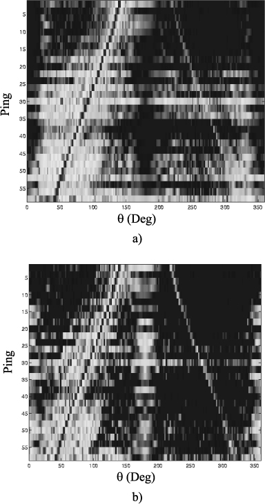
Figure 13.10. Port-starboard rejection ratio (dB)
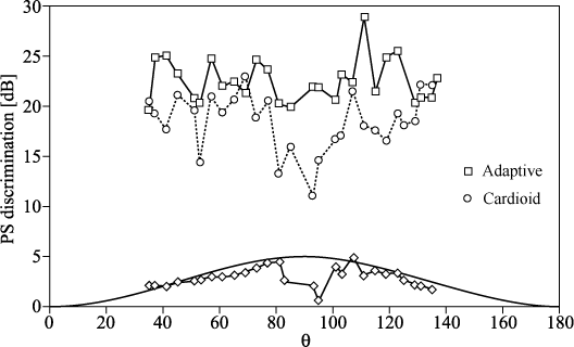
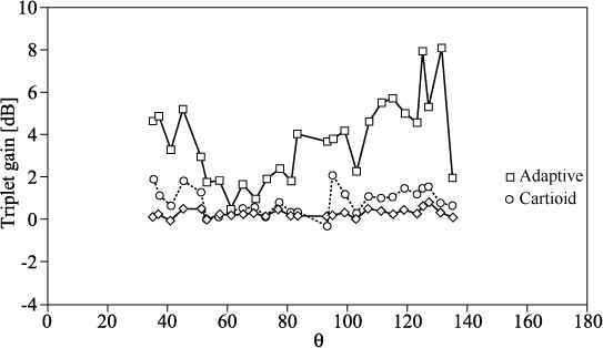
Figure 13.11. Gain (dB)
For each ping, the range data slice (or bearing cuts) containing the target has been selected and the successive cuts are completed. Level dynamic range is identical on the two displays, and the processing is normalized with respect to the signal (gain of 1 on the target in both cases).
It can be seen that the noise level is reduced in case of adaptive beamforming and that the port-starboard rejection ratio is larger. The ghost (or ambiguous target) is more visible at the adaptive beamforming output, which is due to the reduction of the output noise level.
Values of the port-starboard rejection ratio (20log(r)) and gain G measured for the two beamformings versus ping number are shown in Figure 13.11.
13.2.4. Conclusion
Detection and port starboard discrimination performances of a triplet linear towed array have been studied theoretically and experimentally in the case of low ratio diameter/wavelength. Triplet array combined with port-starboard adaptive beamforming combines rejection and detection gain. Port-starboard rejection ratios of 30 dB have been measured and additional gain of port-starboard beamforming ranges from 0 to 5dB according to conditions.
13.3. Adaptive beamforming on a triplet array for reverberation reduction
13.3.1. Introduction
We discuss in this section the application of the adaptive beamforming described in Figure 13.6 to active sonar in Doppler mode, considering either CW (continuous wave) waveforms or wideband Doppler waveforms (“PTFM” type), of duration T. The reader will refer to [DOI 08] for an introduction to the various active sonar modes and their performance in reverberation. We consider the case of a linear receiving array aligned with its own constant speed V. The target is assumed to be moving, with an absolute radial speed large enough to be in “Zone B” (exo-clutter situation). In this mode the detection performances are related to side lobe rejection, and significant gains are expected from adaptive beamforming. This situation is similar to the airborne radar case.
The main challenge is to obtain enough independent snapshots for the estimation of the covariance matrix. Reverberation in Doppler mode has a spatial structure which depends on the frequency, and also on time as the spatial structure of the environment is not stationary. The interference associated with reverberation in each Doppler channel can be considered as arising from an angular sector of width Δu=λ/(VT), expressed in the variable u=cosθ. For a linear array of length L, taking into account the resolution of the bearing beamforming (equal to λ/L), the reverberation can be considered as arising from an angular sector of ![]() jammers, whose central direction depends on frequency. The number of degres of freedom required to cancel this interference is of an order 2 to 3J. The number of independent snapshots available depends on the mode and array directivity:
jammers, whose central direction depends on frequency. The number of degres of freedom required to cancel this interference is of an order 2 to 3J. The number of independent snapshots available depends on the mode and array directivity:
– in the CW mode, each time slice of duration T (pulse length) will provide one independent snapshot and the number of independent available snapshots per jammer and per pulse duration is:
![]()
– in wideband Doppler mode (PTFM), each slice time of duration T will potentially provide BT/N snapshots, the number of independent available snapshots per jammer and per pulse duration is:
![]()
where λ0 is the center wavelength. Taking into account the typical pulse durations T, the covariance matrix estimation duration can hardly be extended further than a few pulses, and for adaptive beamforming to be effective, Scw and Sptfm should be larger than one. Wideband Doppler waveforms allow us to increase this number by an order of magnitude with respect to CW.
As the number of sensors on the array is in the range of several hundred, the adaptive beamforming must be implemented in beamspace domain in order to drastically reduce the number of degrees of freedoms [DOI 10]. It can be implemented either after conventional beamforming, by selecting the appropriate beams steered on the reverberation sectors as noise references (beam space beamforming), or at the output of conventional beams formed on selected sub-arrays from the full array (sub-array beamforming).
Figure 13.12 shows an example of a Doppler bearing plot of the energy at output of the conventional (Figure 13.12a) and adaptive (Figure 13.12b) processing for a sin2 weighted CW pulse. Adaptive sub-array beamforming described in Figure 13.6 was implemented at the output of replica correlation. The acoustic length of the triplet array was close to 20 m, for an external diameter of 80 to 90 mm. The covariance matrix was estimated over several successive independent snapshots in time. The parameter VT/L was equal to 0.52.
Figure 13.12. a) Conventional beamforming on one sub-array; b) adaptive port-starboard beamforming
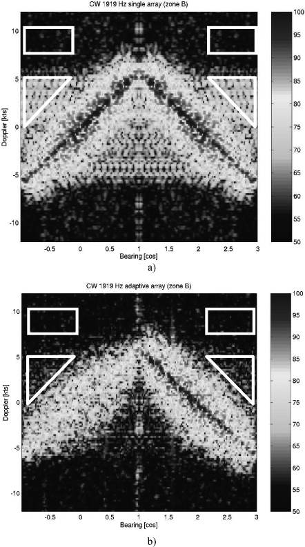
The reverberation leaking through the sidelobes is clearly visible in Zone B in conventional processing (Figure 13.12a). It has been reduced almost to the level of the background noise through adaptive processing. Measured gain in signal-to-reverberation ratio averaged at 18 dB on this example.
13.3.2. Conclusion
The results presented in this section show the benefit of adaptive array processing in active sonar, in strongly non-stationary reverberation dominant conditions. These results were obtained through a drastic reduction of the number of degrees of freedom by implementing beamspace adaptive beamforming, while taking into account the physics of the encountered situation. These results show a very strong analogy with the case of airborne radars in the presence of surface clutter. The processing described here can be considered as a simplified version of space-time adaptive processing (STAP), where adaptivity is reduced to the spatial dimension to provide a trade-off between convergence and performance.
13.4. Bibliography
[BEE 05] BEERENS S.P., BEEN R., GROEN J., DOISY Y., NOUTARY E., “Adaptive port-starboard beamforming of triplet arrays”, IEEE Journal of Oceanic Engineering, vol. 30, no. 2, p. 348–359, April 2005.
[CAP 70] CAPON J., GOODMAN N.R., “Probability distributions for estimators of the frequency wavenumber spectrum”, Proc. of the IEEE, October 1970.
[DOI 95] DOISY Y., “Port-starboard discrimination performances on activated towed array systems”, Proceedings of Undersea Defence Technology, Cannes, France, p.125–129, 1995.
[DOI 08] DOISY Y., DERUAZ L., VAN IJSSELMUIDE S.P., BEERENS S.P., BEEN R., “Reverberation suppression using wide band Doppler sensitive pulses”, IEEE J. of Oceanic Engineering, vol. 33, no. 4, October 2008.
[DOI 10] DOISY Y., DERUAZ L., BEEN R., “Interference suppression of subarray adaptive beamforming in the presence of sensor dispersions”, IEEE Transactions on Signal Processing, vol. 58, no. 8, August 2010.
[SPE 71] VAN DER SPEK G.A., “Detection of a distributed target”, IEEE on A.E.S., vol. 7, no. 5. September 1971.
1 Chapter written by Yves DOISY.