
Chapter 14
Airborne High Precision Location
of Radiating Sources1
14.1. Introduction
Sensors onboard military aircraft must provide a large number of functions. For instance for radar, functions include search, tracking, and ground imagery (SAR); while electronic warfare functions include search, identification and location of transmitting sources, counter-measures, etc.
One possible solution is to assign one antenna to each of these functions. However, this leads to a great increase in antennas numbers and to implementation problems due to the small number of possible antenna locations on a combat aircraft. Furthermore, the implementation of an increasing number of antennas on an aircraft may impact its aerodynamic performances, and also cause an increase in its radar cross-section. Future designs will probably rely on conformal, broadband antennas. Such designs will yield new benefits: enlarged field of view, simplified radomes, higher antenna gain when large surfaces can be used, and will probably imply sharing one single antenna between various functions (i.e. radar + electronic warfare + communications on a single broad band antenna).
However, this design leads to some specific problems: antenna integration to aircraft skin, complex wiring, problems which are presently addressed by the various manufacturers. Another crucial problem arises: being implemented closely to aircraft structure, antennas are submitted to various deformations and vibrations coming from the platform. In the case of an antenna array, positions of antenna elements will no longer be known with enough precision, leading to degradation of antenna performances. Large arrays are quite sensitive to this problem.
ONERA has been conducting research into this topic for about 10 years, mainly in the framework of an internally funded project which ended in 2006. For a year, ONERA has been working on a DGA funded project in the field of ESM (electronic support measures), its aim being to evaluate a flying demonstrator. Besides these projects, ONERA was involved in multilateral cooperation and contributed to the work of NATO Research Groups, namely: SET-060/RTG20 Smart Antenna Structures from the years 1999 to 2002, SET-087/RTG50 Vibrating Antennas to 2006, and presently SET-131 Vibration Control and Structure Integration of Antennas, which started at the beginning of 2009.
During these years, ONERA first undertook theoretical studies in order to understand the physics of mechanical vibrations, their impact on antenna functions and the performances of compensation methods. Later on, ONERA conducted two lab experiments in an anechoic chamber in order to consolidate the theoretical analysis. One of these two experiments is reported in this chapter.
Problem formulation is first introduced in section 14.2. Description of a lab experiment, undertaken at ONERA in 2005 is given in section 14.3: we first describe the experiment itself, and the implemented compensation methods. We then present results produced by this experiment. Finally, section 14.4 concludes this chapter.
14.2. Problem formulation
Let us first remark that the problem of vibrating antennas is multidisciplinary: structure dynamics will deal with platform vibration assessment and modeling, knowledge on various sensors is mandatory if they are to be used to measure platform vibrations; flight dynamics will facilitate platform movement simulation, antenna modeling will assess antenna-structure coupling phenomena, and signal processing will help the understanding of antenna performance degradation due to antenna displacement, and assessing compensation methods performances. ONERA’s expertise covers all of these different fields.
It is important to note that the problem of vibrating antennas on airborne platforms covers a wide range of situations. Each situation is a special case; however, we try to give general rules in the following.
If we want to know whether vibrations/deformations degrade a particular function, we have to consider not only the antenna itself and its function, but also the platform. Performance degradation actually depends on operating frequency, on bandwidth, on processing integration time, and on the nature of the function itself.
Actually, for a given deformation amplitude, performance degradation will be more severe at high frequency than at low frequency, just because the reference is the signal wavelength λ. A 1 mm deformation corresponds to λ /30 at 10 GHz, that is to say 12° of phase error, and to λ/300 at 1 GHz, or 1.2° phase error.
Instantaneous bandwidth and integration time must be related to correlation time of vibrations or to their spectral characteristics. Information on this data can be obtained from aeronautical standards, such as the French “GAM-EG 13” which gives maximum acceleration values on generic platforms. We understand that performance degradation depends on the platform itself (deformation/vibration level and their spectral characteristics), and furthermore on the particular place where the antenna is implemented.
It is well known, that, except for resonances, vibration spectrum decreases with frequency. For a rather “rigid” platform such as some combat aircraft, this means that vibrations will be encountered, rather than static deformations; vibration frequencies will go up to several 100 Hz, but with low amplitudes. On the other hand, in the case of a flexible platform such as a MALE UAV (medium altitude long endurance unmanned airborne vehicle) for instance, mode frequencies will be lower, but amplitudes quite higher. In the case of a given function, impact will thus be very different.
During ONERA project lifetime, impact of vibrations and deformations on antenna performance was investigated with a parametric approach. Various compensation methods using signal processing [WEI 89, WEI 95, MAR 93], were also tested. These methods generally use signals of opportunity, present in the antenna environment.
Using these signals, and if all of them are transmitted by sources of unknown location, it is possible to estimate antenna shape except for a rotation because the system “antenna + sources of opportunity” will give identical received signals whatever the rotation. As most of the time the antenna position must be known relative to the aircraft, we have to bring forward some other assumptions: for instance, [WEI 89] uses knowledge of the position of 2 particular antenna elements. Another possibility is to use signals transmitted by sources with known locations.
Generally speaking, we can think of 3 different techniques for deformation/vibration compensation:
– Active control can keep vibrations under a maximum level, by imposing direct forces on the antenna structure; it can be used in the case of vibration amplitudes that are not too large, present on a antenna that is not too wide.
– Mechanical or optical sensors can help to measure deformations.
– Processing of known signals can be used as explained below.
For cost reasons, the experimental part of the ONERA project was oriented towards a receiving antenna (ESM application) which had 2 advantages: a simpler implementation (mainly compared with radar), and the possibility of testing several compensation methods. We thus considered a receiving antenna onboard the “BUSARD” aircraft, a motor glider used as a test-bed for ONERA experiments.
Two different reasons led us to this choice. The first is a cost reason: BUSARD is an available and cheap platform to operate. The second reason is a limitation found during the theoretical part of our work: simulation of deformation and vibrations on a given platform implies not only having a finite element code at one’s disposal, but also inputs for this code, describing the mass and stiffness distribution of the inner structure. This data is very difficult to get, since it is kept confidential by aircraft manufacturers for obvious reasons. In the BUSARD case, it was possible to restore some main characteristics from simple data.
We thus considered the case of an array antenna implemented on the BUSARD platform in order to test compensation methods studied by simulation during the first part of the project. We considered a receiving antenna, used for direction finding. A preliminary lab experiment was conducted in 2005, in an anechoic chamber. Its description is given in the next section. This experiment allowed us to test 2 of the 3 methods mentioned above, active control being obviously not suitable for our large array antenna. The two methods implemented for antenna shape estimation were a mechanical method based on the use of strain gauges, and a second one based on the processing of signals coming from known sources.
14.3. Description of lab experiment
14.3.1. Context
We want to simulate a platform flying over a theater. Its antenna is used for direction finding, with the final aim of estimating radiating sources, location on the ground. As illustrated in the next figure, we simulate a large interferometer made of two linear sub-arrays disposed along the fuselage and the wing of the platform. In this context, the main task is thus to estimate antenna positions with a precision allowing us to keep location performance close to what is obtained in the case of a perfectly known antenna.
Figure 14.1. 2D interferometer array on BUSARD motor glider (artist view)
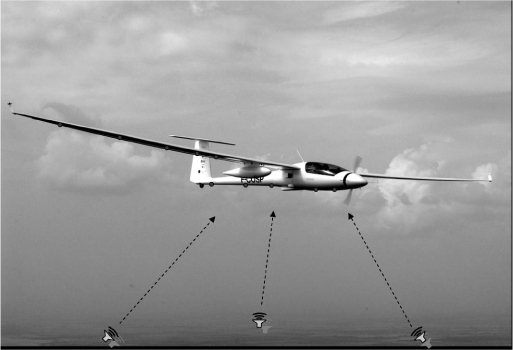
In this figure, array elements are represented by little circles. Note that during real flights, pods will be removed.
In order to simplify the experimental setup, narrow band signals were considered. Carrier frequency was chosen equal to 1 GHz. In a real application, receivers have a large instantaneous bandwidth, but most signals can still be considered as narrow band.
As mentioned above, two compensation methods were tested:
– The first one directly uses some RF signals transmitted by sources of known location and received by the array, and was proposed by the Electromagnetism and Radar Department (DEMR).
– The second one uses signals generated by strain gauges disposed along a subarray; a structure model allows us to estimate antenna shape from these signals. This method was proposed by the Aeroelasticity and Structural Dynamics Department (DADS).
14.3.2. General principle
14.3.2.1. Compensation methods
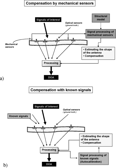
The first method uses known signals (Figure 14.2b), while the second method uses signals provided by strain gauges (Figure 14.2a). The following two sections give more insight into these methods.
During the experiment, optical sensors were implemented near each antenna, in order to measure their real position as a function of time. The data rate was 2 kHz, and the measurement precision was 50 μm.
Figure 14.2. Compensation methods used during 2005 experiment: a) compensation method using mechanical measurements; b) compensation method based on known location signals
14.3.2.1.1. Use of signals transmitted by sources with known locations
ESM context is rather restrictive for these methods, because most of the samples are used to separate incoming signals in frequency (spectral analysis), thus leading to a small number of samples available for vibration compensation followed by direction finding. Even if several successive measures related to the same transmitter are available, used methods must yield results in real time, with a limited number of samples. In the case of radar signals, samples are available at the rate of the PRI (pulse repetition interval), which can lead to a rather slow refreshing rate compared with the vibration frequency. For instance, for a vibration mode with a 10 Hz frequency (100 ms vibration period), we will get only 60 snapshots in the case of a radar PRI of 1.5 ms. If it is necessary to sum the snapshots in order to increase the signal-to-noise ratio, to have better performance of the compensation method, only a few snapshots can be considered as in a static case. If too many are summed, they are related to different shapes of the array that will lead to a “mean shape” estimation and bad performance of compensation.
In this context, iterative methods must be avoided, although some are very efficient [WEI 89]. We thus implemented the simplest and fastest solution, based on direct inversion of the equation linking measured signal phases to antenna positions.
For given antenna positions, the array receives signals coming from different sources, each corresponding to a different arrival direction. Given “ ns ” is the number of received sources, the received phases for all received signal can be written as:
[14.1] ![]()
and:
![]() ; is a ns × 3 matrix;
; is a ns × 3 matrix;
Vds = [us,vs,ws] is the steering vector of source “s” (1 × 3);
![]() is a nc × 3 matrix of antenna positions (x , y , z);
is a nc × 3 matrix of antenna positions (x , y , z);
nc is the number of antenna elements;
Pi = [xi, yi, zi] = is a line vector 1 × 3 containing the coordinates of antenna “i”;
φ is a ns × nc matrix containing the received phases from the ns sources.
By definition, positions P0 of antenna at rest (non-distorted array) are known. For each reference signal of known direction of arrival, it is possible to write the phase received by the non-distorted array as:
[14.2] ![]()
Of course, phases corresponding to reference sources are measured on the distorted array, with actual positions P:
[14.3] ![]()
Using [14.2] and [14.3], we can express the difference between these phase sets as a function of the variation of antenna position due to platform deformation:
[14.4] ![]()
where:
![]()
![]()
Displacements may then be estimated by:
[14.5] ![]()
where Vdref is a nsref × 3 matrix containing the steering vectors of the nsref known sources.
![]()
It is worth noting that the matrix inversion is only possible if we have as many known sources as dimensions to be estimated. Thus for 3D displacements on antenna elements, 3 known sources are needed. Furthermore, the distribution of directions of arrival in space is an important factor influencing the precision with which antenna shape will be estimated. Signal-to-noise ratio is of course also a determinant factor. So, compensation efficiency depends on the number of reference sources, their angular position and their power, which will impact the procedure leading to the choice of reference sources to be used, if there are more sources than the required minimum number.
14.3.2.1.2. Antenna shape estimation using strain gauges
In this case, we used the SPA (strain pattern analysis) method; this method uses the mathematical relationship existing between structure deformations and measurements produced by any mechanical sensor, through knowledge of mode shapes of the structure. Thus, this method relies on the mechanical measurement of displacements as well as on the exploitation of a structure model.
The drawback of this method is that it depends on the quality of a structure model which is initialized by way of a computation performed by a modeling code, most of the time a finite element structure model. Afterwards, this theoretical model has to be adjusted by using ground vibration tests, which is the expertise of DADS department of ONERA.
This method relies on two general principles of structure dynamics:
– Every shape, at time t, can be expressed as a linear combination of mode shapes Φij of plane structure, weighted by generalized coordinates qi. The knowledge of generalized coordinates and dominant mode shapes within strain thus allows us to rebuild displacements on selected points. For example, the displacement z at time t and on j point, expresses as:
![]()
the summation performed, theoretically based on an infinite number of modes, is practically limited depending on the nature of solicitations (application point(s), spectral content), of observation and of measurements precision;
– The vector of generalized coordinates is common to all representative quantities of dynamic observations. Particularly, concerning displacement measurements as well as local strain measurements, we can express that: z = Φdq and ε = Φεq, where z is the displacement measurement or proportional to displacement, e is the strain measurement or proportional to strain, and Φd, ε is the eigenvector matrix of displacements or strains.
Therefore, if we know how to obtain the vector of generalized coordinates, by strain measurements (using strain gauges for example, as in the SPA method), we have easy access to displacement, by projection on physical coordinates: ![]() . The main problem is of course the inversion of the strain matrix Φε, whose size must be at least equal to the number of selected modes (full rank matrix). Actually, simulations confirm that it is necessary to know the shapes measured by gauges with a better precision than for displacement shapes.
. The main problem is of course the inversion of the strain matrix Φε, whose size must be at least equal to the number of selected modes (full rank matrix). Actually, simulations confirm that it is necessary to know the shapes measured by gauges with a better precision than for displacement shapes.
However, as the displacements z are generally expected to be obtained on a limited number of points, it is theoretically possible to reduce the size of eigenvectors of matrix Φd only to the number of those points. Nevertheless, a greater number of points can enable improvement of shape and orthogonality by smoothing for example, or by means of any other process included in modal analysis software. Ground tests are therefore very important, because they not only allow us to correct the initial (theoretical) model, but also allow us to measure mode shapes Φd, ε. We must also keep in mind that the SPA method is limited due to sensor precision, as well as model precision.
This method has been applied in the past by DADS department of ONERA to helicopter blades, and therefore has been tested in the framework of current experimentation.
14.3.2.2. Direction finding with antenna shape estimation
In the case of a non-distorted array, whose elements positions are perfectly known, the direction finding process consists of a minimization of the distance between measured phases and phases stored in a reference table. For a distorted array, 2 extra steps are necessary (steps 1 and 2 below):
– estimation of element positions using reference signals or strain gauge signals;
– correction of the reference table corresponding to the non-distorted array;
– minimization of the above mentioned distance, as in the non distorted case.
For each of the 2 approaches tested during the experiment, the main processing steps become as follows:
– Use of reference signals: phases of reference signals allow us to estimate antenna positions, (![]() on the above figure), from which antenna displacements are calculated (with reference to the undistorted array). From these displacements, the reference table in corrected and measured phases can be compared to the updated reference table. Minimization of the distance between the measured phases and those stored in the updated reference table allow us to estimate the direction of arrival of unknown signals.
on the above figure), from which antenna displacements are calculated (with reference to the undistorted array). From these displacements, the reference table in corrected and measured phases can be compared to the updated reference table. Minimization of the distance between the measured phases and those stored in the updated reference table allow us to estimate the direction of arrival of unknown signals.
Figure 14.3. Direction finding with use of reference signals
– Use of strain gauges signals: the algorithm principle remains unchanged, except that the displacements estimated from outputs of strain gauges are used to update the reference table.
Figure 14.4. Direction finding with use of strain gauges signals
14.3.3. Experiment
14.3.3.1. Description
To be representative of the situation shown in Figure 14.1, while firmly fixing and properly deforming the mock-up, the experiment was carried out by rotating the scene by 90°; so the wing of the mock-up is vertical and the fuselage is horizontal.
Figure 14.5. Picture of the BUSARD
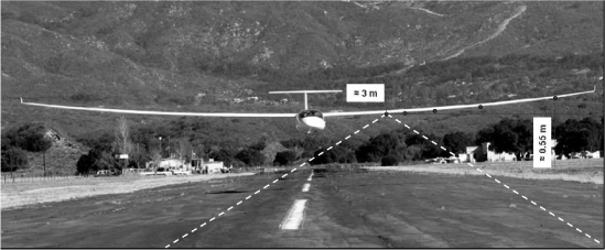
Figure 14.6 below shows a front view of the mock-up, equipped with two arrays with 5 patch antennas (surrounded by white circles) and all the mechanical components. These two arrays operate in receive-only mode.
Note that the array is shifted towards the end of the wing to avoid potential problems of masking due to the fuselage, as shown in Figure 14.5.
Figure 14.6. Picture of the mock-up
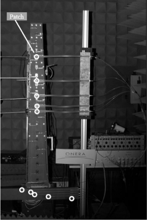
The patch antennas are fed by flexible microstrip lines to conform to the surfaces of the mock-up, but also to tolerate the movement of the array of the wing during deformations. We see on the right of Figure 14.6 that the microwave cables feeding these patches are also flexible for the same reasons. The received signals are translated to baseband and digitized at 60 kHz. The signals are spectrally separated by filtering, and interferometric processing is applied to locate them finely. Then, based on the estimated angles of arrival [θ , ψ] of the received signals, equivalent locations “on ground” are calculated for a given flight altitude, assuming a flat ground.
The deformations are only applied to the wing, which is equipped with mechanical elements allowing:
– activation of static and dynamic deformations;
– the optical and mechanical measurements of the shape of the wing, in front of the antennas. Given that optical measurements are very precise, they give the “true” positions, which are used as a reference when evaluating the accuracy of the compensation methods.
Figure 14.7. Artist view of the experiment
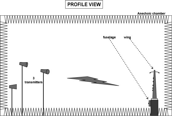
Measurements were performed in an anechoic chamber to minimize external interference and multipath due to wave reflections with the elements surrounding the mock-up. The mock-up faced three emitters centered on three different frequencies in a 30 kHz bandwidth around the carrier frequency F0= 15 GHz. The wing had a length of about 1 m and the arrays had a length of about 50 cm, which represents approximately 23 wavelengths at 1 GHz, taking into account the scale factor.
Transmitters are of continuous wave type, operating near 15 GHz, with constant amplitude (not adjustable). Two of them were fixed and relatively far from the antenna axis. A third transmitter was fixed on a rail controlled by a computer, to have different source positions.
Figure 14.8 shows the scene, viewed from the mock-up.
Figure 14.8. Picture of the three sources
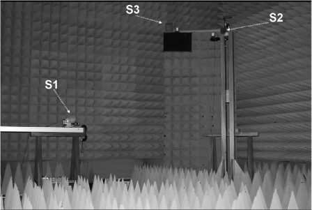
Figure 14.9. Experiment – top view
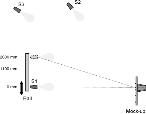
Note that the motion of source S1 on the rail also allows us to have a variable signal-to-noise ratio (SNR), depending on the gain of the antenna of the source in the direction of the array. Thus, it makes it possible to assess the impact of the SNR of known sources on performance of the compensation methods.
14.3.3.2. Results
Measurements were made with high signal-to-noise ratio (SNR = 26 to 34 dB after spectral filtering) in order to visualize firstly the effects of deformations, and secondly the ability of estimating the position of antennas.
In our analysis, we first verified that the localization is effective when the aircraft is not distorted: this is the reference case. Then we looked at various types of deformation, comparing performance with and without compensation. For each configuration, we have evaluated the performance compared to the reference case. For all figures presented below, we can see:
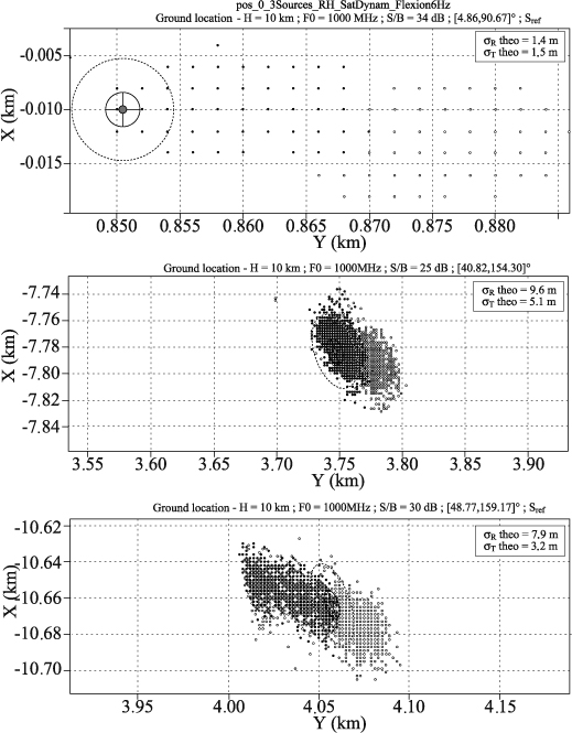
– a plot of the ground location, assuming flat ground and an altitude of 10 km. This location is obtained from the estimated directions of arrival [θ, Ψ] of the received signals. This plot is represented by a cloud of points, corresponding to the estimates computed versus time;
– some ellipses in continuous line corresponding to the 1 σ domain, and some ellipses in dashed line corresponding to the 3 σ domain (each one containing more than 68% and 99% of points if the estimation noise is Gaussian). σ is the standard deviation of the estimated error. Ellipses in thin line correspond to theoretical calculations obtained from three parameters: the size of the array, the direction of arrival of the emitters and their estimated SNR. They represent the performance that should be achieved without distortion. Ellipses in thick line indicate the domains estimated from the cloud of points. The comparison with theoretical ellipses can give an idea of the performance degradation caused by the deformation.
14.3.3.2.1. Performance of localization – reference case
First, it is important to ensure that the 2D interferometry algorithm is efficient. So, we consider the case “without deformation”, and we check that the estimated positions of sources (thick line) correspond to the expected values (thin line). Figure 14.10 shows an example.
We show the estimated location of the three sources, in an axis system centered on the aircraft. The y-axis corresponds to the vector of displacement of the aircraft. By convention, the sources S1, S2 and S3 are represented from top to bottom respectively.
Figure 14.10. Location of sources on the ground – reference case (without deformation)
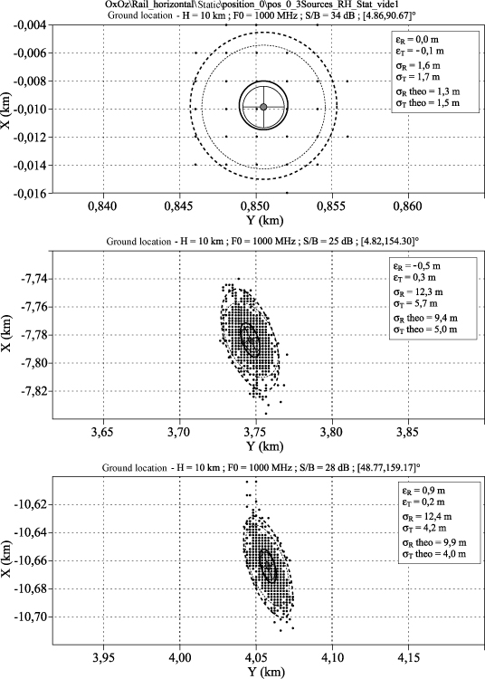
We see that the estimated average error (εR and εT are the radial and transverse components) is almost not biased. Similarly, the standard deviation of the estimated error (σR and σT) is consistent with the theoretical value (σRtheo and σTtheo), except along the radial axis of the sources S2 and S3 for which the SNR has probably been overestimated in the theoretical calculation.
14.3.3.2.2. Performance of localization – effects of deformations on interferometry
Static deformations
In the static case, we considered two deformation levels:
– Level A: around half a wavelength ( λ/2 ) at the ends of the array (i.e. 1 cm at 15 GHz);
– Level B: around 2λ (or 4 cm). Knowing data of the motor glider BUSARD in flight, this level corresponds roughly to the deformation that the array in scale 1, operating at 1 GHz, would suffer.
Unlike the level B, the level A corresponds to a deformation which does not generate phase ambiguities along the array (i.e. phase rotation in the domain [−π +π] ). This level has been considered to assess the ability of the compensation method to estimate the positions of the antennas without having to remove the ambiguities due to the deformation.
For each level of deformation, we obtain the results shown in Figure 14.11.
In the case of moderate static deformations, we see in Figure 14.11a that estimated standard deviations are comparable to the expected theoretical values. But a significant bias is present, in the order of 100–150 m in this case, which cancels the system functionality. It is therefore necessary to compensate for this negative effect.
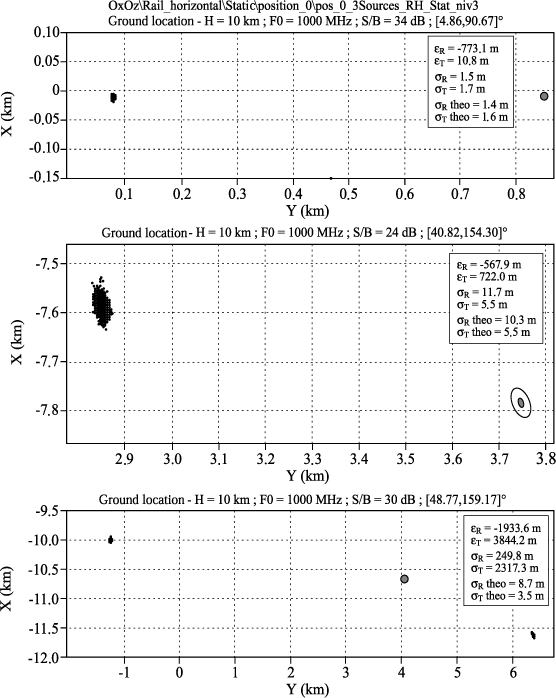
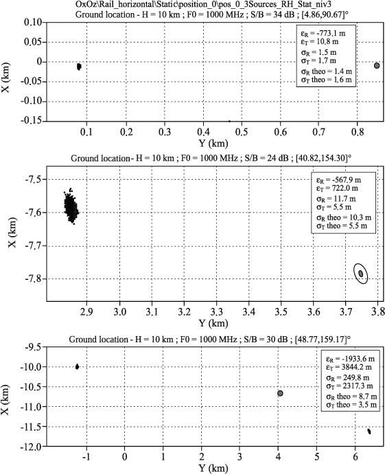
When the deformations are very large (Figure 14.11b), ambiguity problems can be added to the problem of bias. This is the case for the source S3, for which the estimated locations are separated into two areas (clouds, centered at [−10.5, −1.2] km and [−11.6, 6.3] m).
This effect has to be related to the function to ensure. In the present case, the interferometry processing gives very large angular errors when the phase ambiguities are not properly removed. However, this problem makes the compensation more difficult because we must estimate the positions of the antennas in the presence of phase ambiguities related not only to the sparse array itself, but also to the deformation.
Figure 14.11a. Location of sources on the ground: static deformations – level A, without compensation
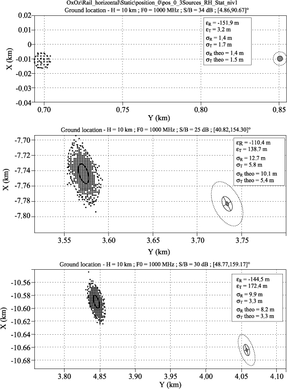
Figure 14.11b. Location of sources on the ground: static deformations – level B, without compensation
Dynamic deformations
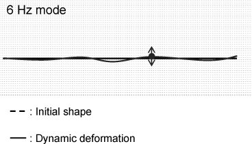
In our analysis, we first considered deformations centered on the reference position (Figure 14.12), by exciting the first mode of fluctuation of the wing, close to 6 Hz.
Figure 14.12. Example of a “centered” dynamic deformation
Then we added a static deformation to this mode of fluctuation in order to have a “static + dynamic” deformation (Figure 14.13).
Figure 14.13. Example of a static + dynamic deformation
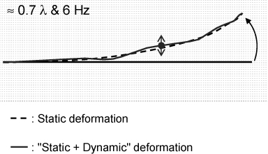
To be as realistic as possible, we should have applied this excitement to a level B deformation, but it was not possible because the risk of mechanical damage of the mock-up was too high. So we considered an intermediate static level of 0.7 λ (between level A and level B), with a dynamic excitation of the 6 Hz mode.
Figure 14.14a. Location on the ground: centered dynamic deformation

Figure 14.14b. Location on ground: static + dynamic deformation
The results are as follows.
We see in Figures 14.14a and 14.14b that the dynamic deformations cause a sharp increase of the standard deviation of the estimated locations, due to the displacement of the antennas over time. In case of centered deformation (Figure 14.14a), the location is also centered, but the ellipses have a different orientation because the distortions affect only the array of the wing.
If dynamic deformations are present around a position different from that at rest, there is of course a combination of both effects (Figure 14.14b): a spread of estimates around a wrong direction.
14.3.3.2.3. Performance of localization – methods of compensation
Concerning the method using the known signals, we assume to know the location of sources S1 and S3 (shown at the top and bottom of the figures), and we want to localize the “unknown” source S2. So this is the source that we must consider to evaluate the performance of the compensation method. However, as a check, we also localize known sources, which gives a performance indicator concerning the estimation of the shape of the array.
Note that although only the wing was deformed, as mentioned earlier, the estimation of the two sub-arrays (wing and fuselage) was performed in the compensation step, in order to take the estimation noise of the antenna positions of the whole array into account.
For the method based on mechanical measurements, the location of the three sources is used to assess the quality of the method.
Figures 14.15a and 14.15b below show the locations obtained from both methods of compensation, in both dynamic cases:
– dark gray: based on the known signals;
– light gray: based on mechanical measurements.
Comparing these results with those of Figure 14.14, we see that both compensation methods can significantly reduce errors. In the case of centered dynamic deformations, we see that both methods give very similar results, particularly for the unknown source S2. In the case of static + dynamic deformation, we have verified that the two clouds are not shifted as it seems in the figure, instead they are superimposed.
The shift relative to one another, and relatively to the true direction, is due to a problem of calibration of the system. In fact, this bias is not inherent to the methods, but is due to the calibration. Indeed, such a calibration has been implemented to correct unknown values of the system. For example, the phase errors due to the receiver chain, but also to the geometry of the scene, need to be corrected. For the latter, we need to know the position of the sources relatively to each antenna. We need also to make a correction from a “spherical wavefront” to a “planar wavefront”, because unfortunately we are here in a near-field situation. However, since the array is deformed, the “right” positions of the antennas are not known and the initial correction “spherical → plan”, when the array was not deformed, is no longer completely valid.
Figure 14.15a. Location on the ground: centered dynamic deformation – with “known signals” compensation and: “mechanical” compensation
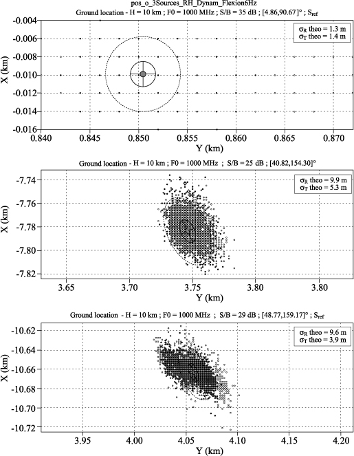
Figure 14.15b. Location on the ground: static + dynamic deformation – with “known signals” compensation and “mechanical” compensation
In fact, to properly calibrate the distorted array, we should know the actual position of the antennas, those we want to estimate. With this paradox, it is normal that a phase error is remaining, which gives a small bias in the localization. This explains why this problem of bias does not arise for centered dynamic deformations.
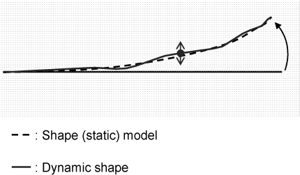
The static cases of Figure 14.14 gave the same trends, so they are not presented. Note however that it was necessary to adapt the compensation method based on known signals in the case of strong deformation (static case, level B). We take into account a “macro” model of deformations in order to cancel phase ambiguities due to large deformations. ONERA’s dynamic structures specialists proposed a simple but sufficiently representative model because there is no need to be perfectly predictive. Indeed the possible inaccuracy of the model is corrected by estimating actual positions, as shown in Figure 14.16. Note that this model accounts for the static deformation of the wing, and is used to remove phase ambiguities caused by it.
Figure 14.16. Artist view of a deformation
Another solution would be to consider displacement measures to remove the phase ambiguities. Just as the model must be sufficiently representative in the previous approach, the measurements must be precise enough, relative to the electromagnetic wavelength. But we have not tested this second approach during the experiment because it was unnecessary. Indeed, Figure 14.15 has shown that the mechanical method is sufficiently accurate (in the cases tested) to provide a measure to be used directly with the table of goniometry. In this case, it is not useful to improve the measurement accuracy by an additional step exploiting the known signals. On the other hand, in another context, this solution might be relevant.
14.4. Conclusion
The work conducted in ONERA’s internal project on the theme of deformable arrays of antennas was useful to have a good idea of the effects of vibrations/deformations of large antenna arrays on the performance of a number of radar and ESM functions.
Overall, it is difficult to generalize the results obtained on a special case both in terms of the effects and the solutions. Of course general rules can be defined, as uncontrolled bad focusing of a deformed array or a rise of the side lobes, etc. But each situation must be studied in detail, depending on the type of aircraft, the function to provide and the locations of antennas on the aircraft. To give a satisfactory response, the levels and the type of vibrations/deformations undergone by the array have to be known, to assess the level of degradation of the function. If the function is no longer performed in good conditions, we must choose or define the compensation method best suited to the constraints given by the aircraft, the antenna array and the function. A study of performance of the methods proposed will be necessary before concluding on the overall effectiveness of the function.
Another general rule we should remember is that the spectrum of acceleration of a structure subject to external stress decreases with its resonance frequency. In other words, a flexible structure will deform more slowly and with greater amplitude than a rigid one. These two concepts, amplitude and speed of deformations, have to be compared respectively to the wavelength of electromagnetic signals and the processing time of the function.
Concerning the experiment described in this chapter, we can conclude that the two means used to compensate for the deformations of a linear array showed a fairly good efficiency. One is based on mechanical measurements of local deformations, based on strain gauges, coupled with a structure model to compute the antennas positions. The other is based on received signals from emitters with known positions (which is quite conceivable in an ESM context). However, the difference between these two approaches should be noted: the precision of the “mechanical” method is proportional to the amplitude of the deformation, while that of the “signal” method is a function of the wavelength, signal-to-noise ratio and position of known transmitters relative to the antennas array.
14.5. Bibliography
[MAR 93] MARCOS S., “Calibration of a distorted towed array using a propagation operator”, J. Acoust. Soc. Amer., vol. 93, no. 4, pp. 1987–1994, March 1993.
[WEI 89] WEISS A.-J., FRIEDLANDER B., “Array shape calibration using sources in unknown locations – A maximum likelihood approach”, IEEE Trans. Acoust. Speech, Signal Process, ASSP, vol. 37, no. 12, p. 1958–1966, December 1989.
[WEI 95] WEISS A.-J., FRIEDLANDER B., “‘Almost blind’ signal estimation using second-order moments”, IEE Proc.-Radar, Sonar Navig., vol. 142, no. 5, p. 213–217, October 1995.
1 Chapter written by Thierry DELOUES, Dominique MÉDYNSKI and Dominique LE BIHAN.