Chapter 1
Joint Diversity and Beamforming for
Downlink Communications1
1.1. Introduction
Mobile communication systems must be able to cope with fading and multi-user interference. Since the introduction of GSM until today, these problems have been considered from different angles and several approaches have been proposed to mitigate impairments.
Digital processing of the signal coming from an array of antennas (called smart antenna techniques) [JAK 74, RAP 01, YAC 93] has played a very important role in the progress achieved in this area so far. Among the novel techniques in this area, we can cite beamforming, diversity and MIMO (multiple input multiple output) techniques as the most successful. Smart antenna techniques can be applied either at the base station or at the mobile, and on the downlink or uplink. For technological and economical reasons, it is often more advantageous to only have an array of antennas at the base station, and a single antenna at the mobile. For the sake of simplicity, but without loss of generality, in this chapter we will consider the downlink of a mobile system with an antenna array at the base station and a single antenna at the mobile.
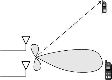
The main goal of beamforming is to increase the signal-to-noise ratio (SNR) at the desired mobile and to reduce the interference generated toward other mobiles present in the system. This is done by directing the radiated signal towards the receiver. The chosen direction does not necessarily match the geographical direction, but can correspond to the main path of the electromagnetic waves traveling from the base station to the receiver.
Figure 1.1. Beamforming directs the radiated signal towards the desired mobile
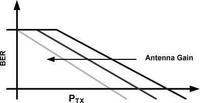
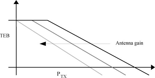
By forming a beam in the direction of the mobile, the transmit power (PTX) can thus be reduced in order to maintain the same bit-error rate (BER). The amount of transmit power saved in the process is called antenna gain. In fact, the effect of beamforming can be seen as a shift of the BER curve to the left.
Figure 1.2. The antenna gain provided by beamforming allows us to obtain the same BER for a reduced transmit power (PTX). The performance curve is thus shifted to the left
The diversity approach treats the same problem from a different perspective. When looking closer at the propagation channel between the base station and the mobile receiver, we notice that this channel is generally formed by the sum of several smaller paths (called multipaths). Each multipath is characterized by its attenuation, delay and relative phase. These parameters vary in time due to the relative motion between the transmitter and receiver, but also due to the movement of all reflectors and obstacles present in the surroundings.
Hence, the overall propagation channel seen by the receiver is the result of the sum of all the multipaths, which translates into a time variation of the signal power at the receiver. This effect is the so-called fading. When the phases of the multipaths are such that they lead to a destructive combination (a strong attenuation of the transmit power), we talk about deep fading.
In practice, the performance of the mobile systems is highly degraded by the presence of deep fadings. The mitigation of these deep fadings is thus the main goal of the diversity techniques. The central idea is to exploit the fact that the channel shows a low correlation to send copies of the same signal, which will suffer uncorrelated attenuations. Thus, the probability that all these copies encounter a deep fading at the same time is very low. Therefore, by combining these copies at the receiver, we can drastically reduce the probability that the received signal is in deep fading and, even in the rare cases when it occurs, the duration of the fading is also diminished.
To best profit from diversity, the copies transmitted by uncorrelated multipaths should also be uncorrelated among them. In this manner, the receiver can combine these copies in such a way as to result in the addition of the multipaths’ powers, leading to the best use of the transmitted power at every time instant.
The different multipaths correspond to the diverse uncorrelated modes over which the signal can be transmitted, and the number of modes is called the diversity order of the channel. These modes are characterized in different domains, respectively in the spatial domain by the direction of arrival (DOA), in the temporal domain by the delay, and in the frequency domain by the selectivity. When the multipaths are uncorrelated in the temporal domain, we say that the channel provides time diversity. In the same way, when the multipaths are uncorrelated in the frequency domain, the channel provides frequency diversity. Instead, the use of an antenna array introduces a new processing domain and, therefore, a new kind of diversity that exploits the spatial decorrelation among multipaths, called space diversity. The use of the space diversity is of fundamental importance in mobile communication as it allows for an overall diversity order greater than 1, even when the channel is flat in frequency (no frequency diversity) and is time invariant (no temporal diversity).
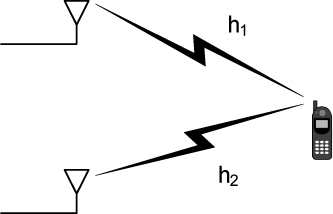
Figure 1.3. Space diversity: the transmitter uses two uncorrelated multipaths to communicate with the mobile
The use of space diversity makes better use of the transmit power (PTX) in the probabilistic sense, leading to a reduction of PTX for the same BER. The slope of the BER curve becomes steeper with the diversity order of the channel. The relationship between the actual slope and the slope obtained without exploiting the channel diversity is called the diversity gain.
Figure 1.4. The use of space diversity leads to the same BER with a reduced transmit power (PTX). The slope of the performance curve becomes steeper
1.2. Space diversity versus beamforming
The assumptions behind beamforming and space diversity are contradictory. On the one hand, the best results for space diversity are obtained when the channels between each antenna and the mobile are uncorrelated. On the other hand, in order to best exploit the antenna gain provided by beamforming, these channels must have a minimum amount of correlation.
In practice, the physical channel between the base station and mobile user is never completely correlated or fully uncorrelated. The correlation depends strongly on the environment and on the antenna geometry. A way to affect this correlation is to build the antenna array in order to have correlated (or uncorrelated) channels with a high probability [SUV 01].
We can roughly say that each technique has a preferred utilization domain. In the low SNR region, beamforming is the natural choice to improve the link performance. On the contrary, in the high SNR region, performance is mostly degraded by fading, so that space diversity brings better improvements. Figure 1.5 illustrates this idea of disjoint application regions as a function of the SNR.
Figure 1.5. Beamforming and transmit diversity application regions
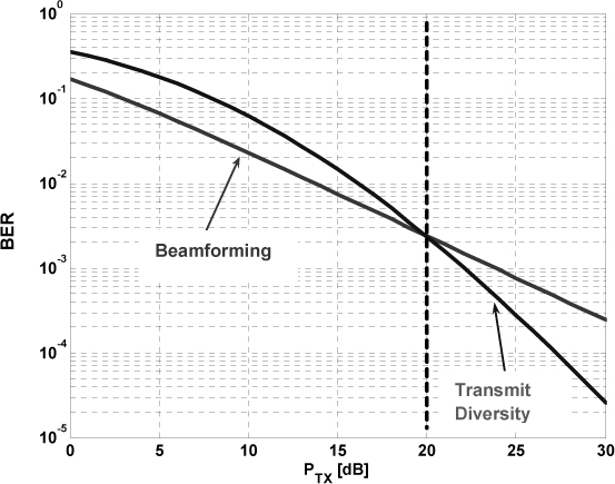
The threshold (vertical bold line in Figure 1.5) between both regions is not easily obtainable and must be adapted to the particular transmission conditions. Thus the need to find adaptive algorithms to automatically choose the best strategy to be used or, ideally, to best combine both strategies.
1.3. Signal model
We consider the downlink of one cell of a wireless communication system, where the base station (BS) is equipped with M antennas and the mobile user (MU) has only one antenna. The signal is transmitted in blocks of Nb symbols, so that the channel variation within one block of data is negligible. However, the channel can change from one block to another, characterizing a block-fading channel.
Let s(b,n) be the signal to be transmitted at time instant n within block b. The signal at the m-th antenna output at the BS is given by:
[1.1] ![]()
where * represents complex conjugate and wm is the coefficient of the purely spatial filter, responsible for the transmit beamforming.
The received signal by the MU can be expressed as:
[1.2] ![]()
where hm (b) is the complex coefficient that links the transmitting antenna m to the receiver antennas, and v(b,n) is the additive Gaussian noise sample at the MU antenna.
By inserting [1.1] in [1.2], the received signal can be written as:
[1.3] ![]()
The expression between the parentheses is the gain of the effective channel between the BS and the MU and can be written in vector form as:
[1.4] ![]()
where w and h(b) are column vectors, defined as w = [w1 w2 … wM]T and h(b) = [h1(b) h2(b) … hM(b)]T. Moreover, we consider the beamforming vector w to be normalized, i.e. |w| = 1.
By observing that the first term in [1.4] corresponds to the useful signal and the second term corresponds to noise, we can write the average received power by the MU during block b as:
[1.5] ![]()
or:
[1.6] ![]()
Without loss of generality, assume that the symbols s(b,n) have power PTX, ![]() . Thus, equation [1.6] becomes:
. Thus, equation [1.6] becomes:
[1.7] ![]()
where R(b) is the instantaneous downlink channel covariance matrix (DCCM), given by R(b) = h(b)h(b)H. The term instantaneous stresses the fact that it only considers the channel at block b.
Note that, for each block b, the channel h(b) can be in a different condition, i.e. it can be in a deep fading condition or in a condition that favors the transmission. Hence, the received power may vary considerably from one block to the next.
1.4. Beamforming by SNR maximization
The SNR seen by the MU during block b is given by:
[1.8] ![]()
where ![]() is the noise power v(b, n), assumed to be stationary.
is the noise power v(b, n), assumed to be stationary.
The maximum SNR criterion for a fixed transmit power can be written as:
[1.9] 
with the constraint ![]() w
w![]() = 1.
= 1.
In [1.9] the expectation is carried on different blocks b, since the channel varies from one block to another. The average DCCM is given by R = E{R(b)}.
By introducing the Lagrange multiplierλ the Lagrangian associated with [1.9] can be written as:
[1.10] ![]()
The subscript “mono” highlights the fact that we consider here a single user case, as opposed to a multi-user case.
[1.11] ![]()
Therefore, the optimum beamforming wopt is the eigenvector of ![]() , corresponding to the eigenvalue λ.
, corresponding to the eigenvalue λ.
By multiplying the left hand side of [1.11] by wH, we have:
[1.12] ![]()
We note that λ corresponds to the SNR to be maximized, which implies choosing the eigenvector associated with the maximum eigenvalue in [1.11].
Finally, we can write:
[1.13] 
In the wireless communication context, the beamforming solution according to the maximization of the SNR has the disadvantage of being based on average values (signal power and noise power) and not considering the variation of these values in time, due to fading. This comes from the use of the covariance matrix R, which reflects the mean behavior of the channel, but does not contain any information about the variation of the instantaneous power P(b). However, the BER is extremely sensitive to the variations of SNR (due to the variation of received power). This fact comes from the relationship between SNR and BER, given by ![]() where the function Q(.) is nonlinear and convex.1
where the function Q(.) is nonlinear and convex.1
It seems obvious that beamforming, using a purely spatial filter and based on the maximization of the SNR, cannot mitigate fading since this technique does not profit from the channel diversity. Thus, we propose here to use several spatial filters in order to create uncorrelated virtual antennas to exploit the channel diversity. This technique is presented in the next section.
1.5. Combining transmit diversity and beamforming
With the goal of combining transmit diversity and beamforming, we propose to cascade a (classical) transmit diversity technique with a precoder. The diversity stage transforms the signal to be transmitted s(b,n) into L “coded” signals ![]() to
to ![]() . These signals are then applied, in the precoder stage, to L spatial filters, w(1) w(2) … w(L). Each of these layers w(k) of the precoder beamforms the signal
. These signals are then applied, in the precoder stage, to L spatial filters, w(1) w(2) … w(L). Each of these layers w(k) of the precoder beamforms the signal ![]() but also scales its power.
but also scales its power.
In a classical transmit diversity approach, the signals ![]() would be transmitted simply using different antennas. In the proposed structure, we say that these signals are transmitted by virtual antennas.
would be transmitted simply using different antennas. In the proposed structure, we say that these signals are transmitted by virtual antennas.
The following figure depicts the proposed structure.
Figure 1.6. Structure combining transmit diversity and beamforming
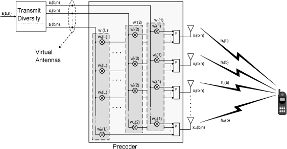
In this case, the signal received by the MU is given by:
[1.14] ![]()
where x(b, n) = [x1(b, n) x2(b,n) … xM(b,n)]T is the vector containing the antennas’ outputs and h(b) = [h1(b) h2(b) … hM(b)] T is the spatial channel vector that links the BS and the MU.
The vector x(b, n) can be written as:
[1.15] ![]()
where ![]() is the signal applied to the virtual antennas and
is the signal applied to the virtual antennas and ![]() is the 1-th layer of the precoder. x(b, n) can be written in matrix form as:
is the 1-th layer of the precoder. x(b, n) can be written in matrix form as:
[1.16] 
Finally, the signal received by the MU is given by:
[1.17] ![]()
with  which is the precoding matrix, also called the precoder. This precoder is normalized so that
 ![]() . This normalization ensures that the power issued to the antenna array is the same as the power of the signal s(b,n).
. This normalization ensures that the power issued to the antenna array is the same as the power of the signal s(b,n).
We can think of the precoder W as a transformation applied to the channel h(b). By posing ![]() as the virtual channel that links the virtual antennas to the MU, [1.17] becomes:
as the virtual channel that links the virtual antennas to the MU, [1.17] becomes:
[1.18] ![]()
The instantaneous covariance matrix of the virtual channel ![]() can thus be written as:
can thus be written as:
[1.19] ![]()
And the average covariance matrix as:
[1.20] ![]()
Equation [1.20] shows that the matrix ![]() is obtained by the transformation of R by the precoding matrix W. The question now is how to choose this precoding matrix to best exploit the channel diversity.
is obtained by the transformation of R by the precoding matrix W. The question now is how to choose this precoding matrix to best exploit the channel diversity.
1.6. Minimum variance criterion
1.6.1. Criterion formulation
A first solution corresponds to minimizing the variation of the received power. This variation is indeed due to fading and its minimization may lead to better performances.
We introduce a column vector w, containing M x L elements, formed by stacking the columns of the precoding matrix W :
[1.21] ![]()
Consider now the convolution matrix H, whose columns are formed by the vector h(b) shifted M rows at each column, given by:
[1.22] 
Using this new notation, the received signal can be written:
[1.23] ![]()
The useful received power at block b is then given by :
[1.24] ![]()
Regardless of the transmit diversity technique used, we consider the virtual symbols ![]() to be i.i.d. (independent and identically distributed) as the symbols s(b, n) are also i.i.d. Moreover, the virtual symbols have the same power PTXas s(b, n). We can thus write:
to be i.i.d. (independent and identically distributed) as the symbols s(b, n) are also i.i.d. Moreover, the virtual symbols have the same power PTXas s(b, n). We can thus write:
[1.25] ![]()
Let us introduce the space-time instantaneous DCCM H(b) of, given by R(b) = H(b) H(b) H. The received power can be rewritten as:
[1.26] ![]()
The proposed criterion is then to minimize the variance of the received power with respect to a target value Pc . The cost function to be minimized is:
[1.27] ![]()
Without loss of generality, we can consider Pc = 1, which leads us to:
[1.28] ![]()
Note that the above criterion is similar to the one that leads to the constant modulus algorithm (CMA), often used in blind equalization.
By a quick inspection of the cost function, we note that minimizing [1.28] can lead to a transmission power value that is too high. Hence, we propose to introduce another term to the cost function which consists of a weighting of the transmit power. The final proposed cost function is then given by:
[1.29] ![]()
where the weight β controls the importance given to the minimization of the transmit power compared to the minimization of the variance of the received signal. The algorithm developed to carry out the optimization of [1.29] is called the constant power algorithm (CPA).
1.6.2. Simulation results
We compare the proposed CPA solution with the classical beamforming, classical transmit diversity and the so-called eigen-beamforming [ZHO 03], which is optimal in the case of Rayleigh fading.
We consider a simple scenario where the BS is equipped with a linear array of 4 antennas with ![]() spacing. The precoder is composed of 2 layers (L=2).
spacing. The precoder is composed of 2 layers (L=2).
1.6.2.1. Non-line-of-sight scenario
The non-line-of-sight scenario consists of a single path at 0° and an angular spread Δ. This is a flat-fading Rayleigh channel.
We consider here Δ=5°, which corresponds to a relatively high spatial correlation. In practice, the value of Δ depends on the distance between BS and MU and on the obstacles that surround the MU.
The eigen-beamforming technique consists of switching from beamforming (diversity order 1) and a full diversity solution (diversity order 2) based on the SNR. This technique always leads to the best BER in this scenario and will be used as a benchmark.
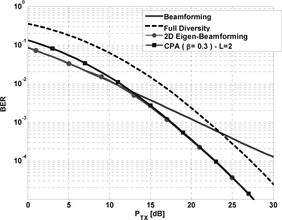
Figure 1.7 shows that the full diversity solution achieves a diversity order of 2, given that the slope of the BER curve versus SNR is -2. This technique distributes the transmit power equally between the two transmit modes of the channel.
The CPA solution presents the same performance as the eigen-beamforming for PTX > 15 dB . Below this value, it would be needed to modify the weighting β in order to better exploit the directivity (beamforming) by putting more weight on minimizing the transmit power instead of the received variance.
Figure 1.7. Comparison between different solutions in a non-line-of-sight scenario
1.6.2.2. Line-of-sight scenario
In order to highlight the advantage of the proposed CPA solution compared to the eigen-beamforming solution, we now consider a non-Rayleigh channel, composed of two multipaths, a direct and a diffuse multipath. The direct path is modeled by a Rice distribution with KRice = 20 dB and the diffuse path is modeled by a Rayleigh distribution. The DOA of the direct channel is 0° and it is 6 dB stronger than the diffuse channel, whose DOA is 40°.
Table 1.1. Line-of-sight scenario parameters
The simulation results show that the CPA solution leads to the best performance in this case, as shown in Figure 1.9. This is explained by the fact that this solution concentrates the transmit power in the direction of the direct path, in opposition to eigen-beamforming, which uses the diffuse path with the same power, as depicted in the radiation patterns below.
Figure 1.8. Radiation patterns for the simulated techniques in the line-of-sight scenario
Indeed, both layers of the CPA solution radiate mainly in the direction of the direct path, but they also radiate in the direction of the diffuse path with different phases, which explains the better performance achieved by this technique when compared to beamforming. The beamforming solution tries to maximize the (mean) received power by radiating in the direction of both multipaths. Since the direct channel almost has a constant module, the use of the diffuse path can only degrade the performance since the combination of both multipaths creates fading. The same is true for the Eigen-Beamforming solution, developed for the Rayleigh channel and no longer optimal in the conditions of this experiment.
Figure 1.9. Comparison between different solutions in a line-of-sight scenario
1.7. Minimum BER criterion
1.7.1. Criterion formulation
The minimization of the variance of the received power was proposed with the goal of reducing the BER at the receiver. Let us now directly use the BER expression in the cost function to be minimized. Recall that the SNR at the block b is given by ![]() . Hence, the BER of block b, at relatively high SNR can be approximated by:
. Hence, the BER of block b, at relatively high SNR can be approximated by:
[1.30] 
where N is the number of bits per symbol, dmin the minimum distance between 2 points for a unitary power constellation, ![]() is the mean number of neighbors at this minimum distance, and the function Q(.) is given by:
is the mean number of neighbors at this minimum distance, and the function Q(.) is given by:
Since the term ![]() is constant, it can be omitted from the minimization and the minimum BER criterion JmBER (w) can be written:
is constant, it can be omitted from the minimization and the minimum BER criterion JmBER (w) can be written:
[1.31] 
1.7.2. Simulation results
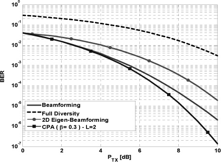
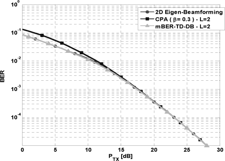
In the context of a non-line-of-sight transmission described above, the algorithm which optimizes the minimum BER criterion, named mBER-TD-DB, achieves the same performance as the eigen-beamforming approach, as shown in Figure 1.10.
Figure 1.10. Comparison between different solutions in a non-line-of-sight scenario
The algorithm minimizing the BER can be easily applied to different cases, as shown by the extension to the multi-user case in [ZAN 09, ZAN 10]. We consider in the following a scenario with two MU and two multipaths between each user and the BS. The parameters of this scenario are summarized in Table 1.2.
Table 1.2. Two-path scenario parameters
The classical multi-user beamforming (i.e. based on the minimization of SNIR) solution is shown in Figure 1.11, where we observe that each radiation pattern “points” in the direction of one user.
Figure 1.11. The radiation pattern obtained with the classical multi-user beamforming technique. Two user and two path scenario
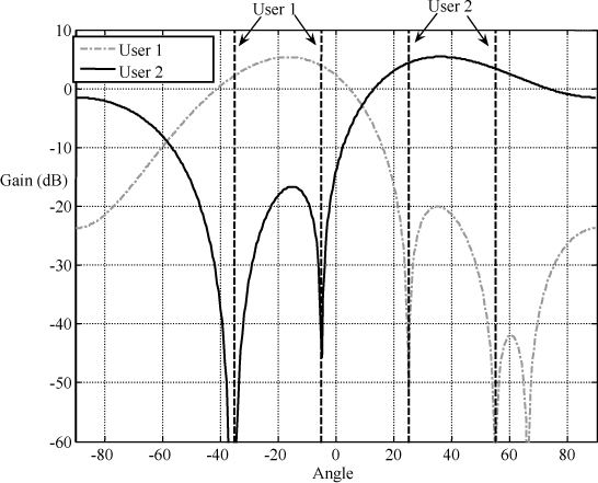
Figure 1.12. Radiation patterns for user 1 obtained with the minimum BER algorithm. Two user and two path case, using a two layer precoder (L=2)
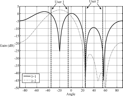
Figure 1.12 shows the result obtained with the proposed algorithm based on the minimization of the BER. We observe that both layers of the precoder radiate in the direction of the first user without interfering with the second user. Moreover, each layer radiates in a different manner toward the first user, which is required to exploit the spatial diversity present in the channel. By doing so, the minimum BER technique is capable of jointly performing beamforming and transmitting diversity in a multi-user case.
1.8. Conclusion
In this chapter two techniques to jointly perform beamforming and diversity on transmit have been presented. They both have the goal of minimizing the received BER at the mobile unit for a given transmit power at the base station. The first technique, called the constant power algorithm (CPA), is based on the minimization of the variance of the received power. The performances of this technique are equivalent to the eigen-beamforming technique [ZHO 03] for Rayleigh-distributed flat-fading channels. For all other channel types, the CPA solution leads to better performances than the eigen-beamforming technique. The performance of the CPA technique depends on the adjustment of the parameter β, which controls the weight given to beamforming with respect to transmit diversity. In order to circumvent this problem, we have proposed a second solution, directly based on the minimization of the BER. This technique can adaptively adjust the trade-off between beamforming and diversity to obtain the minimum BER. Moreover, it can be extended to the multi-user case, allowing us to jointly perform transmit diversity and multi-user beamforming.
1.9. Bibliography
[JAK 74] JAKES W.C., Microwave Mobile Communications, IEEE Press, New York, 1974.
[RAP 02] RAPPAPORT T.S., Wireless Communications: Principles & Practice, Prentice Hall, 2nd edition, New York, 2002.
[SUV 01] SUVIKUNNAS P., VAINIKAINEN P., HUGL K., “The comparison methods of different geometric configurations of adaptive antennas”, Proc. of the 4th European Personal Mobile Communications Conference (EPMCC'01), Vienna, Austria, 2001.
[YAC 93] YACOUB M.D., Foundations of Mobile Radio Engineering, CRC Press, Boca Raton, 1993.
[ZAN 09] ZANATTA-FILHO D. et al., “Adding diversity to multiuser downlink beamforming by using BER constraints”, submitted to European Transactions on Telecommunications, November 2009.
[ZAN 10] ZANATTA-FILHO D., Nouvelles méthodes de traitement d’antenne en mission: Alliant diversité et formation de voie pour les systèmes de communication radio-mobile, Éditions Universitaires Européennes, 2010.
[ZHO 03] ZHOU S., GIANNAKIS G.B., “Optimal transmitter eigen-beamforming and spacetime block coding based on channel correlations”, IEEE Transactions on Information Theory, vol. 49, no. 7, pp. 1673–1690, July 2003.
1 Chapter written by Luc FÉTY, Danilo ZANATA-FILHO, João Marcos TRAVASSOS ROMANO and Michel TERRÉ.