
Chapter 17
Anti-jamming for Satellite Navigation1
17.1. Satellite navigation principles
17.1.1. Triangulation
The GNSS (global navigation satellite systems) include any systems of radio navigation by satellite. The only GNSS operational is the US GPS (Global positioning system), and at a lower scale the Russian system (GLONASS, fewer operational satellites). Other GNSS systems are under construction like the European system GALILEO, but also the Chinese system (COMPASS/Beidou). These systems allow every user using a GNSS receiver to determine his navigation parameters (3D position, 3D speed and time) regardless of time or place.
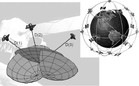
Navigation by satellites is based on the triangulation principle. It consists of calculating the position of a receiver by estimating the distance between this receiver and 3 GNSS satellites (Figure 17.2), enabling us to resolve the 3 unknowns of the position: latitude, longitude and altitude.
The distance d between the receiver and every satellite is calculated by estimating the propagation delay of the signal from the satellite to the receiver. The emission time is known thanks to the very precise clocks installed on satellites, and transmitted in the signal via the message of navigation broadcasted by every satellite; the reception time is known thanks to the internal clock of the receiver. The distance d is thus proportional to the propagation delay (at the speed of light c):
Figure 17.1. Galileo constellation [MAG 06]
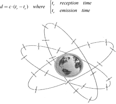
Figure 17.2. GNSS triangulation
However, as the satellite and receiver clocks are not synchronized, a 4th unknown must then be considered: the time bias. The receiver will thus need at least 4 satellites to resolve its 4 unknowns and determine his position and time.
17.1.2. GNSS signals: the GPS example
The GNSS use signals modulated in band L. Considering the example of the current GPS, 2 frequencies are used: L1 = 1,575.42 MHz and L2 = 1,227.60 MHz. Furthermore, GPS signal uses multiplexing by code (CDMA – code division multiple access), every satellite having its own code c(t) (also called PRN – pseudorandom noise). Finally, the data D(t) broadcast in the message of navigation is modulated by the PRN code (at lower rate, 50Hz), which leads to the generation of the signal for the code C/A (coarse acquisition) of the system GPS.
Figure 17.3. GPS C/A code generation
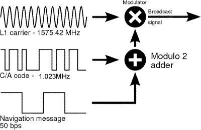
Modulation of the carrier (L band) by the PRN code is a BPSK modulation (binary phase shift keying). The type of code differs according to the applications (opened or military). Presently, two codes are used:
– The C/A code (coarse acquisition) contains 1,023 bits, with a period of 1 ms (frequency of 1.023 MHz), in band L1 only.
– The P(Y) code (precise) reserved for the US and allied armed forces, with a frequency of 10.23 MHz and possessing a period of one week. It is encrypted by the W code to form the Y code. It is present in band L1 and L2.
Figure 17.4. GPS frequency bands
The codes used for the CDMA are chosen because of their good intercorrelation properties. For a code corresponding to a given satellite:
– the autocorrelation presents a maximum in zero and very weak values anywhere else;
– the intercorrelation with the other codes (emitted by the other satellites) is very weak regardless of the shift between the codes
Furthermore, the codes rates (1.023 MHz or 10.23 MHz) allow a spreading of the signal spectrum. To track the signal, the receiver realizes the correlation between the received signal and a local copy of the code. When the received and local codes are in phase, a peak of energy is detected, enabling tracking of the satellite.
Figure 17.5. Correlation of local and received code
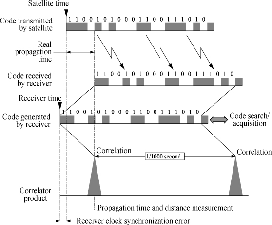
Obtaining a peak of correlation allows us to know that the received code is synchronized with the locally generated code. The dating of this peak of correlation by the receiver thus allows us to know the time of reception tR of the signal. The time of emission tE (position of the code in the time, the beginning of a sequence of code being synchronized in time by the GPS system) is deducted from the signal decoded at this time and from the decoding of the navigation message (modulated in 50 Hz). This is illustrated in Figure 17.6.
Figure 17.6. Receiver clock synchronization error [PIE 06]
However, the measure of the time of propagation, and thus of the satellite– receiver distance, is not sufficient to determine the position of the receiver: in addition we require knowledge of the exact position of every visible satellite. The data contained in the navigation messages provide this information and are then necessary to compute the receiver position. This data is regularly calculated by ground stations and includes almanacs and ephemeris allowing us to reconstitute exactly the position and the speed of every visible satellite.
The whole chain of emission (codes and messages) is summarized in Figure 17.7.
Figure 17.7. Measure of propagation delay by means of correlation [PIE 06]
Once the local code is synchronized with the received code, the receiver has to calculate the receiver/satellite distance evolutions. The signal processing of the receiver thus includes a tracking loop of the received code.
Another phenomenon intervenes in the tracking of the GNSS signal: the receiver has to adapt to the variations of relative speed between the satellites and the receiver. Indeed, satellites revolve around the globe at a height of 20,000 km with an average speed of 4,000 m/s. On the other hand, in most applications, the receiver may also move. This relative speed between the satellite and the receiver leads to a proportional Doppler effect which produces a significant change Δf in the carrier frequency (L1 or L2):
![]()
Furthermore, as the satellite and receiver clocks are not synchronized, a drift of the clock has to be taken into account. Thus, to correctly demodulate the GNSS signal, the receiver has to calculate this Doppler effect. To this purpose, the signal processing of the receiver implements a 2nd tracking loop on the frequency (or the phase) of the carrier.
When the carrier frequency of the receiver is synchronized with the received signal, the phase tracking loop allows us to compute the Doppler effect, which also includes information to reconstitute the speed of the receiver with regard to every satellite.
17.2. Vulnerability of the GNSS signals
17.2.1. GNSS signal power
The power of the broadcasted GNSS signals is typically around several Watt at the level of the satellites. Considering the free space losses on the route from the satellite to the receiver, the received power is then around −130 dB m, that is 10−16 W! The signal power is thus largely under the thermal noise of approximately −100 dBm in the considered band (≈ −170dBm/Hz by taking into account an average noise factor of 4 dB).
Figure 17.8. Received signal power
In nominal conditions, the signal-to-noise ratio in 1 Hz, also called C/N0. (carrier-to-noise ratio), can be expressed according to the signal level S (in dB) and to the level of noise in 1 Hz, N0 (in dB/Hz):
In the presence of jamming, the signal-to-noise ratio is decreased. It can be expressed using the jammer-to-noise ratio J/S, and the spectral separation coefficient (SSC) which represents the spreading of the jammer in the band:
So, the higher the SSC, the more the jamming is going to impact the receiver. This coefficient is generally expressed as SSC = −10.log10(Q.RC) where Q is a quality factor and RC the frequency of the code. One of the most disturbing jammings is then a sinusoid centered on the specter (Q = 1). If an interference has a “matched spectrum” (same spectrum as the GNSS signal), then Q = 1.5. In the case of a white noise wideband jammer, Q ≈ 2 (see [KAP 05]). The different powers are illustrated in Figure 17.9.
Figure 17.9. Signals power
Figure 17.10 shows the evolution of the signal-to-noise ratio versus the jamming power for the open code (C/A) and the military code (P (Y)) of the GPS system. Even an interference of power equivalent to that of the thermal noise degrades the signal-to-noise ratio. Moreover, the open C/A code is less resistant than the military one. When the power of the interference prevails, the signal-to-noise ratio becomes independent from the thermal noise and follows an asymptote with a slope of 1 dB by degradation of C/No for a 1 dB of increase of J/S. In the first approach, the equation of this asymptote is “70 dB – J/S ” for the P(Y) code and “60 dB – J/S ” for the code C/A.
Figure 17.10. C/No versus interference power
17.2.2. Example of interference scenario
In Figure 17.10 we added, for each code, the levels of interference which make the acquisition and the tracking of the signals impossible.
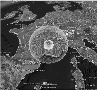
Taking as an example an interference of 20 W placed in Valence (France), we can determine the jammer spheres of influence in the case of civil GPS receivers (C/A code) using a standard omni-directional antenna. The source of interference is located at the center of the spheres. Inside the smaller sphere, any pursuit of GPS signals is impossible. Inside the larger sphere, any acquisition of new satellites is impossible.
Figure 17.11. Interference effect on C/A code
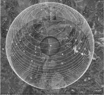
The use of military GPS receivers gives access to the code P(Y) which offers a better resistance to interference, as depicted below in the same jamming and antenna case.
Figure 17.12. Interference effect on P(Y) code
The calculations are simplified and assume a direct visibility between the interference and the receiver. Hypotheses are as follows:
– 20 Watts of jamming power emission with an antenna of 0 dBi1, i.e +43 dBm at the frequency L1 = 1,575.42 MHz.
– Level of the GPS signal = −130 dBm for C/A code, −133 dBm for P(Y).
– Gain of the receiving antenna = +2 dBi.
By using the following formula:
![]()
And under the following hypothesis:
– The limit of acquisition using C/A code of J/S = 24 dB implies a maximum level of interference of −106 dBm, i.e. free space losses of 150 dB, which corresponds to a minimum distance of 550 km.
– The limit of pursuit using C/A code of J/S = 43 dB implies a maximum level of interference of −88 dBm, i.e. free space losses of 133 dB, which corresponds to a minimum distance of 70 km.
– The limit of acquisition using code P(Y) of J/S = 41 dB implies a maximum level of interference of −92 dBm, i.e. free space losses of 137 dB, which corresponds to a minimum distance of 110 km
– The limit of pursuit using code P(Y) of J/S = 54 dB implies a maximum level of interference of −79 dBm, i.e. free space losses of 124 dB, which corresponds to a minimum distance of 25 km
It is thus clear that classic methods of GPS signal processing are vulnerable to interference, and that some applications may require more robust navigation capabilities. A possible answer is the use of non-standard antennas as described in the following sections.
17.3. GNSS antennas
17.3.1. GNSS standard antennas
We deal here with GNSS aeronautical applications, and thus called “standard GNSS antennas ”, antennas classically used in aeronautics. The majority of the characteristics of these antennas are also valid for commercial and mass-market applications with however differences in the form factor, serial price and environment specifications.
GNSS signals being broadcaste by satellites whose positions vary with time, the main function of the standard antenna is to receive as many satellites as possible without any assumption on their direction. Radiation pattern is thus omnidirectional (i.e. isotropic) and ensures quasi-constant gain down to low elevations. It is nevertheless noteworthy that the gain is lower on purpose for low elevations so as to counter multipath effects on navigation performances. Hence a standard antenna may be modeled as isotropic down to about ten degrees of elevation then as having low gain for small elevations and back lobes. Gain for such antennas is typically between 0 dBi to +5 dBi right hand circular polarized. Associated technologies are various (dipoles, spirals, etc.) and depend on the application.
Figure 17.13. Example of standard antenna radiation pattern
Typically patch antennas are used for aeronautical applications because of their compactness and flushness (to reduce aeronautical drag and/or reduce radar cross-section). Patch antenna structure is quite simple with one or more dielectric on top of which a metallic patch is printed. The dimensions of this patch are linked to the reception frequencies to be received.
For civilian applications the C/A code is received only on the L1 frequency while for military applications the P(Y) code is received on both L1 and L2 frequencies. In the latter case, one solution is to have two superposed patches, each resonating at one frequency. Polarization may be achieved by feeding patches in quadrature with a hybrid coupler or by choosing the right place for the feeding point on the two patches.
Figure 17.14. Patch antennas (left), aeronautical antenna (right)
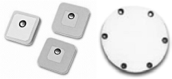
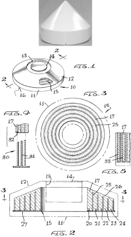
“Choke-ring ” antennas are used for applications of metrology (monitoring of the signals GNSS, for example) where the reduction of multipath is essential. They are much more voluminous than patch antennas because multipath mitigation is obtained by concentric conductive circles. Figures below present, on the one hand, the outside aspect of the antenna, and on the other hand, the internal constitution with these concentric circles.
Figure 17.15. Choke-ring antenna example, photography and internal constitution
17.3.2. Non-standard GNSS antennas
In nominal conditions, satellite signals are received with enough gain and overall noise is also nominal. As a consequence the budget link is correct and the carrier-to-noise of each satellite enables the acquisition, tracking and the overall signal processing necessary to perform the navigation solution.
In jamming conditions, interferences are received in the same way as useful satellite signals because the antenna is isotropic. As a consequence, even if signals are nominally received, received noise is increased by the equivalent power of interferences hence degrading carrier-to-noise ratio (see section 17.2 for details and Figure 17.16 – top – for the diagram).
Non-standard antenna principle is thus to modify the omnidirectional radiation pattern using an optimized pattern (dynamically controlled or not) that maximizes the GNSS carrier-to-noise ratio.
Figure 17.16. Omnidirectional reception (top) with CRPA (bottom)
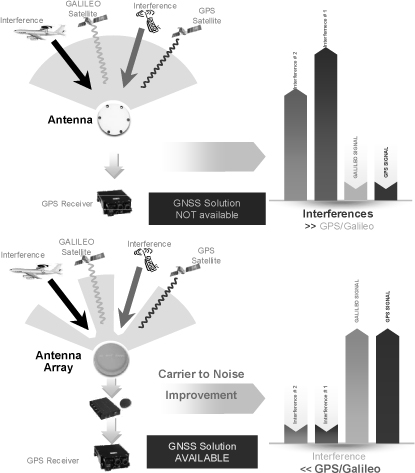
One possible solution is to receive nominally useful signals while minimizing gain in the direction of interferences: we speak then of interference nulling. The generic term for such a technique is CRPA that stands for controlled radiation pattern antenna (Figure 17.16 – bottom). It opposes the acronym FRPA that is associated with standard antennas and stands for fixed radiation pattern antenna.
Beyond interference nulling, it is also possible to adapt the radiation pattern so as to improve the gain in the direction of desired satellites: this is referred to as beamforming:
Figure 17.17. Beamforming reception
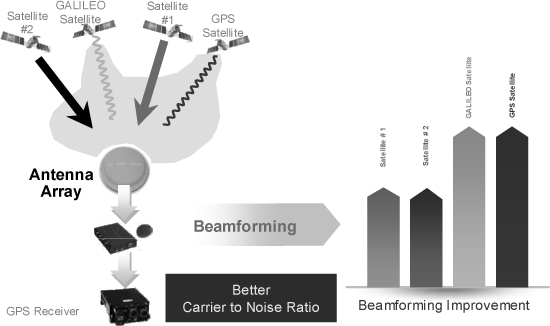
It is of course possible to use the two techniques at the same time so as to improve gain in the direction of useful signals while placing nulls in the direction of interferences.
17.3.3. Equipment upgrade
Such performance improvements rely on a modification of the standard GNSS reception chain. It is classically constituted of one omnidirectional antenna followed by a low noise preamplifier and a GNSS receiver.
Figure 17.18. Standard reception chain

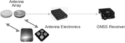
To allow radiation pattern adaptation it is necessary to replace the standard antenna (FRPA) with an antenna array and to replace the low noise preamplifier with antenna electronics that play the same role and null interferences. Available antenna arrays are numerous and the choice is based on form fit constraints and requirements. The upgraded GNSS navigation chain is then more robust to interferences.
Figure 17.19. Anti-jamming reception chain
17.4. Anti-jamming principles
The general description of GNSS principles and standard antennas has shown non-standard antennas interest to improve performances and navigation solution availability. The following sections focus on associated models and derive nulling and beamforming algorithms with key performances. Finally, a list of possible implementations of algorithms is provided.
17.4.1. Space processing
We will set up the equations that are useful for modeling the CRPA processing based on the simplest case (space only array processing).
The principle of the process has already been described above and consists of generating an equivalent antenna pattern starting from an array of antennas, each antenna output being weighted in amplitude and phase. Figure 17.20 models the system as an N antennas array (4 in the figure), every antenna being followed by an adjustable complex weighting. All the weighted outputs are then summed to generate the equivalent antenna pattern that nulls the jammed directions.
Figure 17.20. Principle of space processing
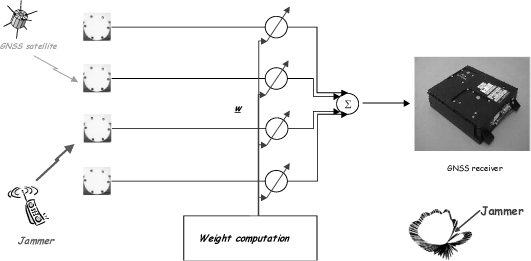
The problem thus consists of reducing the influence of jammers knowing that the useful signal is hidden in the thermal noise. It is considered that any dominating signal in front of the thermal noise is a jammer and that the problem is solved by “simply ” minimizing the equivalent antenna (sum of the weighted antennas) total output power.
17.4.1.1. Data model
Let us consider an array of N sensors illuminated by radio waves originating from various sources distributed in space. Let us also assume to be in a homogeneous medium, so that the propagation velocity C is constant, and the distance from the sources is sufficiently large so that the wavefront received by the array is planar.
Under these assumptions, for a source emitting a monochromatic wave with pulsation w, the received signal at the instant t at the point with coordinates ![]() can be written as:
can be written as:
[17.1] ![]()
where k is the wave vector whose norm is given by ![]() and λ = c/f is the wavelength.
and λ = c/f is the wavelength.
For current GNSS antenna arrays, noting B the signal bandwidth and D the inter-sensors spacing, the ratio BD/c is about 1/100. Thus the narrowband assumption is generally verified, it results in:
[17.2] ![]()
which makes it possible to consider that the time for the wavefront to cross the array is negligible in front of the reverse of the bandwidth of the signal so that the amplitude and the phase of the baseband signal does not have time to vary. Under this assumption, the time delay between the sensors of the array can be approximated by simple phase shift: if τ stands for the time delay and s(t) is the baseband signal, then computing the Fourier transform leads to:
[17.3] ![]()
where the frequency deviation Δf around the carrier frequency fc is less than half the bandwidth of the signal. Thus, by introducing the narrow band assumption, we obtain:
[17.4] ![]()
Finally, calculating the inverse Fourier transform gives:
[17.5] ![]()
with wc=2πfc.
Figure 17.21. Definition of the angles
Thus, if we consider an array with sensors located at coordinates (xk, yk, zk) in an reference system (O, x, y, z) and a source with an elevation angle θ and an azimuth angle (φ(see Figure 17.21), then the propagation delay τk can be written as:
[17.6] ![]()
Hence the received signal at sensor k is:
[17.7] ![]()
where bk(t) is the thermal noise, which is spatially and temporally white. Consequently, if we define:
[17.8] 
with a the array steering vector, we can write the narrow band model that will be used thereafter in the following vectorized form:
[17.9] ![]()
The received signal thus carries information on the position of the incoming signal via the angles θ and φ. Operationally phase shifts are measured compared to a reference sensor, the origin of the axes is placed on this sensor.
The steering vector a(θ) is a function of one or several parameters depending on the array geometry. θ is then either the scalar θ, or the vector θ = [θ; φ] T. If the sensors are assumed to behave linearly, then following the superposition principle, the array output in the presence of p sources with respective directions θ1, …,θp can be written:
[17.10] ![]()
or in vectorized form:
[17.11] ![]()
With:
[17.12] 
We finally define the correlation matrix:
[17.13] ![]()
Thus, assuming that the signals are random processes, uncorrelated with the thermal noise and uncorrelated between each other, we can obtain:
[17.14] ![]()
with ![]() . We have also admitted that the added noise τ2 is spatially white, i.e. uncorrelated between the sensors. The matrix component R(k,l) measures the spatial correlation between the outputs of the sensors k and l.
. We have also admitted that the added noise τ2 is spatially white, i.e. uncorrelated between the sensors. The matrix component R(k,l) measures the spatial correlation between the outputs of the sensors k and l.
17.4.1.2. The power minimization solution
The problem model being written, we just have to solve it as a simple optimization problem: the non-standard antenna must minimize the total output power by calculating a complex weighted sum of the elementary sensor outputs. Let z denote the array output and w be the complex weight vector, then:
[17.15] ![]()
The output power can then be written:
[17.16] ![]()
[17.17] ![]()
In order to avoid the trivial solution where the weight vector would be the null vector, the problem is moved to a constrained minimization problem. The constraint is designed so as to define the non-standard antenna pattern in the absence of a jammer. Indeed, in that case the weighting vector is directly proportional to the constraint c. This constraint may be directional, in this case the antenna pattern in the jammer free case is a beam steered toward the constrained direction. Or the constraint can also be like c = [0 … 0 1 0 … 0]T. In this case, a single elementary sensor is used in the absence of interference. Any other intermediate solution is also possible.
The power minimization problem can be written:
[17.18] ![]()
Solving it using the Lagrange multipliers method leads to:
[17.19] ![]()
then, we obtain:
[17.20] ![]()
By inserting the constraint wHc = 1, we find ![]() or equivalently
or equivalently ![]() . Finally, introducing this term into [17.20] gives:
. Finally, introducing this term into [17.20] gives:
[17.21] ![]()
[17.21] indicates that the weight vector calculation is based on the inverse of the spatial correlation matrix. From a practical point of view, this matrix is not available. Nevertheless, it is possible to estimate it. Various strategies of implementation are possible from iterative methods up to “snapshots ” methods that imply a higher computation load but that are more efficient.
17.4.1.3. Synthetic antenna
The correlation matrix together with the weight vector can be rewritten in a way so as to exhibit the synthetic antenna resulting from the power minimization process.
The idea is to perform an eigenvalue decomposition of the correlation matrix:
[17.22] 
Rewriting the weight vector in a more general way gives:
[17.23] 
The equivalent synthetic antenna created by the treatment thus corresponds to the “subtraction ” to the signal of the reference sensor (imposed by the constraint of the optimization algorithm), that of the sensors forming beams towards the dominating sources with respect to the thermal noise. The algorithm weights each beam proportionally to the ratio between the eigenvalues of the interference and of the thermal noise: the more powerful the interference is, the more the algorithm rejects it.
The eigenvalues decomposition can also be rewritten so as to differentiate between the interference subspace, on the one hand, and the noise subspace, on the other hand:
[17.24] ![]()
Thus, [17.24] reveals p eigenvalues/eigenvectors associated with the interferences and those associated with the thermal noise whose values are identically equal to σ2.
Figure 17.22. Example of eigenvalues distribution
The more complex the environment, the higher the number of degrees of freedom consumed. Figure 17.22 shows eigenvalues associated with various jamming environments (from one single narrowband jammer to several narrowband and wideband combined jammers). We can also note in Figure 17.22 the effect of the use of the estimated matrix instead of the true matrix on the distribution of the eigenvalues of the noise (dispersion around the theoretical value of 0 dB).
17.4.2. Space-time processing
Going from space processing to space-time processing (STAP) is mostly driven by the need of more degrees of freedom (dof). This increase in dof translates in an improvement of wideband interference nulling and in auto calibration (correction of analog impairments) to a certain extent.
Figure 17.23. Principle of the space-time processing
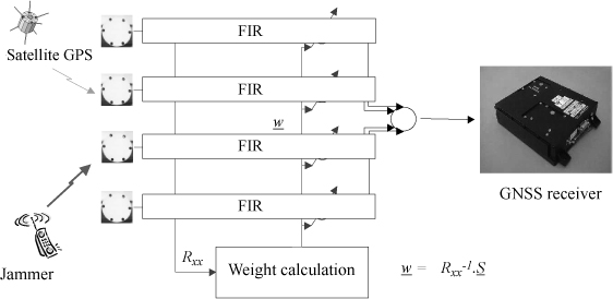
In practice, dof increase is achieved by the replacement of the complex tapering of each antenna in space processing by a finite impulse response filter (FIR). STAP improves nulling performances while increasing computation requirements.
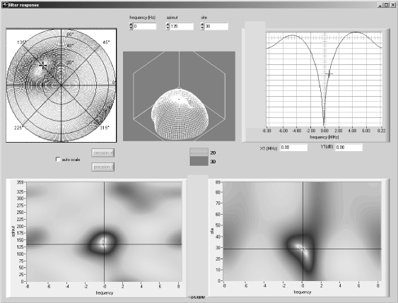
Space-time processing allows interference nulling both in the space domain (azimuth, site) and the time (equivalently frequency) domain. Figure 17.24 shows the processing response for a narrowband interference coming from a direction of 135° of azimuth and 30° of site. The processing being space-time four parameters have to be taken into account: site, azimuth, frequency and nulling. Each figure is obtained by fixing one of the parameters:
– upper left, antenna gain for centre frequency in reduced coordinates;
– upper middle, antenna gain for centre frequency in 3D;
– upper right, antenna gain versus frequency for the interference direction;
– lower left, antenna gain versus azimuth and frequency for fixed site;
– lower right, antenna gain versus site and frequency for fixed azimuth.
It shows a nearly optimal gain over most of the radiation pattern, a null in the direction of the interference (shown as a dot in the figures) and a frequency notch in the direction of the interference.
Figure 17.24. Space-time nulling example
17.4.3. Beamforming
17.4.3.1. Goal of beamforming
The array processing techniques presented until now make it possible to transform the standard omnidirectional antenna into an antenna ensuring the mitigation of jammers. In this case, the reception of the useful satellite signals is ensured by default, i.e. no constraint is introduced to improve the reception in a specific direction
Another possible use of the antenna array consists of optimizing the signal-to-noise ratio of the satellites: the goal is then to form beams in the direction of the tracked satellites. The maximum gain is obtained when the phase delays of all the signals of the antennas are compensated for before their summation. The theoretical gain is thus:
![]()
The achieved gain is thus 6 dB for an array of 4 sensors and 8.5 dB for 7 sensors. This improvement in the signal-to-noise ratio is interesting for example for the acquisition of new satellites: the time to first fix is indeed directly related to the signal-to-noise ratio. The metrology applications (ground control stations of the GNSS signals) can also benefit from this additional gain to improve the acquisition of the satellites rising on the horizon or to improve their integrity. Lastly, an increase in the gain of the antennas can enable us to increase the spacing between the ground stations for the same level of performance.
17.4.3.2. Conventional beamforming
This method is commonly denoted “conventional beamformer ” (CB). It consists of adding in phase coherence the signals arriving from the direction of interest. By using the notation of equation [17.8], the weight vector to be applied is:
![]()
where the gain is normalized to 1 in the direction of interest (θ0,ϕo).
The array output can be seen as the output of a space filter. According to equation [17.7]:
![]()
Thus, when a signal is present at the input of the array, the signal to noise ratio (SNR) per sensor is:
and at the output of the beamformer, the signal can be written:
[17.25] ![]()
Hence, when using a conventional beamformer, the achieved signal-to-noise ratio is:
We hereby find the beamforming gain given previously.
It should be noted that the 3 dB beamwidth depends on the geometry of the array but also, for a given geometry, on the direction of interest. Thus, for a d spacing uniform linear array (ULA), the gain of the array is:
[17.26] 
Leading to a 3 dB beamwidth depending on the angle of arrival according to [VAN 02]:
![]()
17.4.3.3. Adaptive beamforming
It is possible to combine the jammers rejection and the optimization of the signal reception in a given direction with adaptive beamforming algorithms.
The theoretical weight vector computation is identical to the case of the jammers mitigation and also utilizes the array correlation matrix: the optimization problem then consists of the minimization of the array output power (jammers cancellation) while ensuring a nominal gain in the direction of interest:
![]()
The only difference comes from the constraint c which is then a true directional constraint associated with the direction d0 = (θ0,ϕo):
![]()
It thus appears possible to form beams in various directions of space without having to recalculate the inverse correlation matrix R−1 each time. The complementary constraint to form these beams simultaneously is to have as many space filters as the number of desired beams.
Finally, the array channel calibration is mandatory in order to form the beams in the steered directions and to get the desired gain in terms of the signal-to-noise ratio.
17.5. Antenna and associated electronics integration
This section gives an overview of antenna arrays and antenna electronics used to perform the algorithms previously described.
First of all we show different types of antenna arrays, then antenna electronics and finally an overview of interfaces and volumes.
17.5.1. Antenna array examples
Several antenna arrays are available as demonstrators or components off-the-shelf. Main parameters include:
– number of antenna elements;
– antenna element characteristics, possibly different between reference antennas and auxiliary antennas;
– array geometry;
– array dimensions.
A trade-off between all these parameters has to be made to ensure:
– amplitude and phase impairments;
– minimization of array aliases by fulfilling Shannon theorem in the spatial domain;
– minimization of coupling between element antennas;
– maximization of antenna array dimensions so as to guarantee better directivity in the case of beamforming.
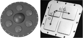
The standard and classical solution involves a 7 antenna version where elements form an hexagon that is a good compromise between space aliases and GNSS satellite availability. An example of such an antenna is presented in Figure 17.25 on the left.
For smaller platforms and/or having less anti-jamming requirements, antenna arrays are limited to 4 elements (nulling up to 3 interferences) placed in a square or “Y ” shape. Such an array is presented in Figure 17.25 right.
Figure 17.25. 7 antenna and 4 antenna array
Several solutions have been proposed to ease integration requirements. As a matter of fact, one of the most important brakes to the wide use of such antennas is their size and weight for small aeronautical platforms, helicopters, etc.
Use of higher permittivity dielectric permits smaller antenna elements at the cost of lower antenna gain. Moreover in any case, narrowing the gap between elements increases coupling leading to performances degradations. Specific techniques are used to deal with such effects.
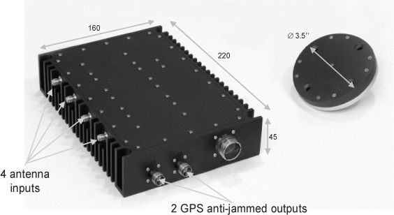
However, solutions are now available at least as demonstrators so that the number of small CRPA available keeps increasing. The standard 7 element antenna array (14″ diameter) is now available in a 7″ diameter version and the 4 element 7″ square is now available in a form-fit equivalent to standard FRPA (i.e. 3.5″ diameter).
17.5.2. Antenna electronics evolution
Historically, first CRPA processing were analog ones, that is to say that tapering was performed by radiofrequency phase shifters in L-band (i.e. 1.57542 GHz and 1.2276 GHz). Analog defaults (components impairments, mismatches between phase command and actual result, etc.) tremendously limit nulling performances of this kind of equipment.
The first demonstrator performing CRPA processing in digital for the GNSS navigation is shown in Figure 17.26.
Figure 17.26. CRPA digital antenna electronics for transport aircraft (2001)
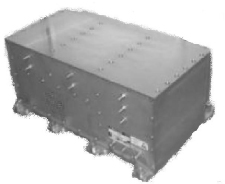
The nulling of interferences was performed in the digital domain, simultaneously on the two GPS bands namely L1 and L2. This demonstrator validated digital space processing and was used for seeking performances limits without size, weight and power (SWaP) constraints.
The next step has been to develop a demonstrator of antenna electronics combined with a GPS receiver including supervisor logic. The supervisors main task was to make the best use of embedded anti-jamming algorithms: space-time processing, on the one hand, and correlation and hybridization techniques relying on inertial and barometric references, on the other hand. This demonstrator named smart receiver is presented in Figure 17.27 with the standard 7 element array.
Figure 17.27. Smart receiver (CRPA+GPS) (2008)
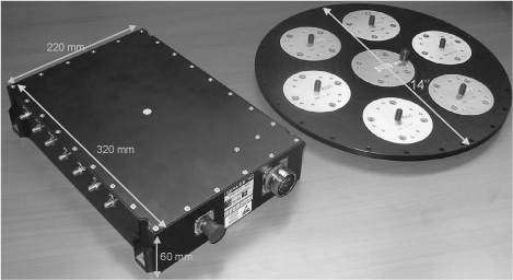
Figure 17.28 shows a small 4 element array (form and fit with GPS standard antenna) with associated antenna electronics.
Figure 17.28. Small CRPA and antenna electronics
17.6. New functions associated with the antenna array
The main requirement for navigation antenna processing is to filter the incoming GNSS signals to ease acquisition and tracking. We have shown before that such processing performs nulls in the direction of interferences and/or beams in the direction of satellites.
In most cases (except conventional beamforming) the algorithm relies on intercorrelation matrix calculation and inversion. It is then tempting to use this information to provide additional services to the final user. For navigation such services include assessment of the number of interferences and with additional calculation burden coarse localization of each of them. The purpose here is not to perform goniometry but to warn the user of the presence of interference that may degrade navigation performances, and to provide a rough localization.
17.6.1. Detection of interferences
The detection of interference presence is quite easy. As already discussed in section 17.2.1, the GPS signal is spread spectrum and the power received is well below the noise level. Hence, as soon as interference is present and adverse it is easy to detect it as its power is well above thermal noise level. By assessing incoming power the receiver is able to detect if interference is present or not and if so to indicate to the final user the interference to the noise power ratio (INR).
By use of the intercorrelation matrix it is also possible to assess the number of interference sources. This information is even more interesting because most localization algorithms rely on it to perform direction finding.
17.6.1.1. Subspace principle
The determination of the number of interference sources is possible by analyzing the intercorrelation matrix defined in section 17.4.1.1. This analysis relies on the splitting into two subspaces (one for noise and another for interferences) by means of eigen-decomposition of the intercorrelation matrix and determination of eigenvalues associated with each subspace.
One example of such a decomposition is provided in Figure 17.29. Eigenvalues are sorted by increasing order, the higher ones corresponding to interferences. One instance of interference may be represented by several degrees of freedom that is to say several eigenvalues. This is the case for wideband interference scenario. This is not an issue as direction-finding algorithms rely on subspace dimensions not on actual interference numbers.
Figure 17.29. Eigenvalues example
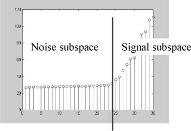
The main issue is to split the eigenvalues into two subspaces, one for noise and another for interferences. In the case of one or several eigenvalue(s) being allocated with the wrong subspace, direction-finding precision is directly impacted. This allocation is even more difficult if interference power is low (interference eigenvalues close to noise ones) and/or complex (for example wideband interference spread over several eigenvalues of decreasing amplitude, the smaller being close to the noise). One solution is to use a robust criterion to assess the number of eigenvalues associated with subspaces.
17.6.1.2. AIC criterion
In practice, the interrelation matrix R is computed over a small number of samples. The idea of the criterion is to use the a priori knowledge of this number of samples to assess the noise eigenvalues spread and optimize the decision threshold accordingly.
One classical criterion is called the AIC that stands for “Aikake Information Criterion ”. It is based on the probability density function of noise eigenvalues spread versus the number of samples used for intercorrelation matrix estimation. One example of noise eigenvalue spread versus sample number is shown in Figure 17.30.
The criterion uses as a priori information the number of antennas (N), the number of taps used by the STAP (P) if space-time processing is used and the number of samples used for matrix estimation (K). One test by possible value of noise subspace rank is performed based on the following cost function:

with:
M: interference eigenvalues number;
L: total number of eigenvalues i.e. degree of freedom (N × P);
K: number of samples;
λi: eigenvalue #i.
The result of the estimation of the number of interferences is the value M for which F(M) is minimum. It is this value that will be used as an input for the direction-finding algorithm.
Figure 17.30. Example of eigenvalues spread versus sample number
17.6.2. Interferences location
Several algorithms may be used to locate interferences. They may be divided into two classes: on the one hand, algorithms that sense power in different directions of space, and on the other hand, high-resolution algorithms that provide better resolution.
In any case, a calibration of analog channels (including antennas) is mandatory and has a direct impact on location performances. Nevertheless, the need for GNSS is not to provide precise direction finding but rather to provide additional situation awareness on interferences.
Several algorithms for interference location [VAN 02] are quickly presented below. The Bartlett method is only presented here as a reference because it does not provide sufficient spatial resolution.
17.6.2.1. BARTLETT method
This method consists of making a beam in each direction of space and calculating the received power. The output mapping provides the direction of space where received power is the most important.
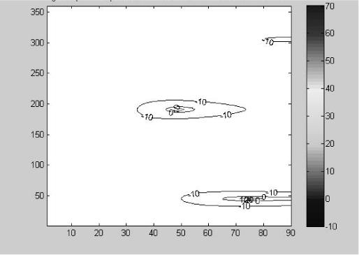
An example of such mapping for a 7 element array with 0.7 wavelengths between antennas is provided for a jammer located at 45° of azimuth and 75° of site with an interference-to-noise ratio of 60 dB in Figure 17.31. The horizontal axis represents site and the vertical axis represents azimuth; measured power is sketched as iso-power curves.
The true jammer direction is shown with a cross actually located in a “high power ” measurement zone (higher than 80 dB) and several aliases are also present.
Figure 17.31. Bartlett method answer for one jammer with a 7 element array
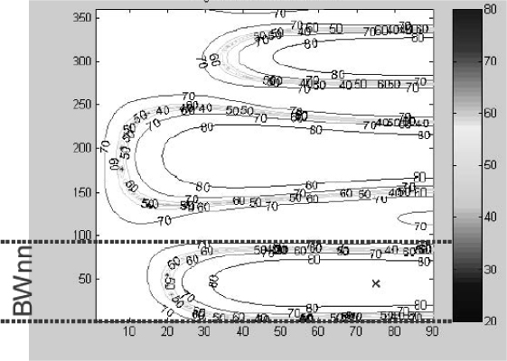
It is also noteworthy in this example that spatial resolution is poor. In fact, it is directly related to the dimension of the antenna array that is “small ” in this case. As a matter of fact, array answer is related to the null-to-null spatial bandwidth (BWnn).This value may be deduced from equation [17.26]. For zenith and a uniform linear array (ULA) with a distance d between elements, it is given by:
![]()
Applying this formula to the 7 element array used for the previous example, leads to a resolution of roughly ± 45°. This is consistent with Figure 17.31 between 0° and 90° of azimuth.
Moreover the spatial answer is poor due to high side lobes (response close to a sinus cardinal, see Figure 17.32 and equation [17.26]).
Figure 17.32. Bartlett method response for two spatially close interferences
For all these reasons this method is not efficient enough to locate interference for GNSS applications.
17.6.2.2. CAPON method
The Capon method provides a better spatial resolution. It does not use the intercorrelation matrix but requires the calculation of its inverse.
Unlike Bartlett's method that is only forming a beam in several directions of space, Capon's method also minimizes the output power of the equivalent antenna.
The basic principle is also to compute the output power in each direction of space and to find maximums in the obtained mapping. The difference comes from array weights that try to whiten the incoming signal thus minimizing the influence of signals coming from directions other than the direction of interest.
Spatial resolution is of the order of a quarter of the 3 dB beam width that is roughly ± 10° for the 7 element array. This is illustrated in Figure 17.33 that corresponds to the same configuration as the one used for the Bartlett method. It is clear that the two interferences are separated showing that the Capon method has a greater spatial resolution.
Nevertheless we must also note that a local minimum is present between the two sources leading to potential issues for identification algorithms.
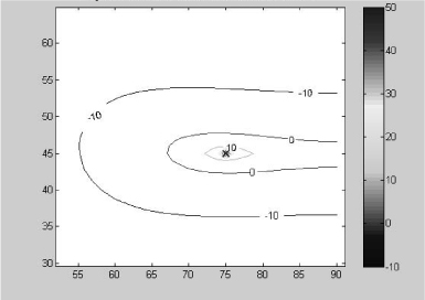
The same interference scenario (7 element array, 0.7 wavelengths, interference located at 45° azimuth and 75° of site) is used to compare Capon and Bartlett's methods. Corresponding mapping is shown in Figure 17.34 and is compared to Figure 17.31. The maximum is sharp in a direction close to actual direction.
Figure 17.33. Capon method response to two spatially close interferences
According to theory the resolution in this case is close to ± 10°, which is consistent with Figure 17.35. Another maximum appears in the figure corresponding to an alias due to array geometry. As a matter of fact, inter-element spacing is larger than half a wavelength.
Figure 17.34. CAPON method response for one interference and a 7 element array
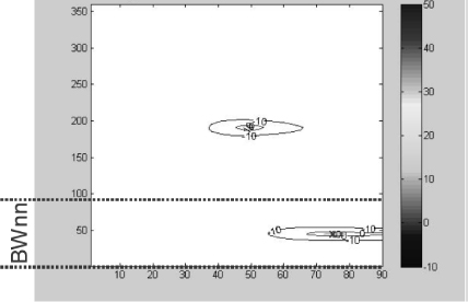
Figure 17.35. Zoom – Capon spatial resolution
17.6.2.3. MUSIC method
This method provides the same order of spatial resolution as Capon's method while supplying more dynamic and robustness in the interference location. It relies on noise and signal subspaces to identify interferences: interference is highly correlated with the signal subspace and de-correlated with the noise subspace (eigenvector orthogonal to noise subspace)
The same scenario as in Figures 17.32 and 17.33 with a ULA and two closely spaced interferences shows that MUSIC outperforms the two previous methods.
Figure 17.36. MUSIC method response to two closely spaced interferences
Finally, the same interference configuration (7 element array, 0.7 wavelengths, interference located at 45° azimuth and 75° of site) is used to compare MUSIC with the two previous methods. The mapping is shown in Figure 17.38 and is compared to Figure 17.31 (Bartlett) and Figure 17.34 (Capon).
Figure 17.37. MUSIC method response to one interference (site: 75°, azimuth: 45°)
The mapping is close to the Capon method, with respect to resolution and maximum locations. MUSIC outperforms other methods (Bartlett and Capon) in dynamic between closed sources and thus in its capacity to efficiently locate such interferences.
17.6.2.4. Min-norm method
This algorithm is based on the same subspace decomposition as the MUSIC method. The main difference is the use of a min-norm eigenvector to span the noise subspace rather than all the eigenvectors as in MUSIC. The underlying idea is that corresponding location performances will be better.
The eigenvector used for noise subspace is a linear combination of all its eigenvectors: it can be shown that this algorithm is a weighted version of the MUSIC algorithm.
This algorithm is able to locate interferences that are weaker than those detected by MUSIC. The drawback is a higher computational burden due to calculation of the weighting vector.
17.6.2.5. ESPRIT method
The last algorithm that we will describe here is called ESPRIT for estimation of signal parameter via rotational invariance technique. It is applicable to antenna arrays that can be decomposed in two identical sub-arrays deducting one another by a known movement. The number of interferences that can be located is then linked to the number of antenna elements of sub-arrays: the decomposition of a 7 element array in two 6 element sub-arrays reduces the number of recognizable interferences from 6 to 5.
Various versions exist including:
– LS-ESPRIT: least-Square ESPRIT, a least-square version;
– TLS-ESPRIT: total least-square ESPRIT, another least-square criterion;
– U-ESPRIT: unitary ESPRIT, which uses a unitary transformation to obtain a real matrix.
The performances of these methods are better than those of MUSIC with an even lower detection threshold.
On the other hand, they allow us to locate fewer interferences (linked to the subarray number of elements) and are very dependent on the geometry of the chosen sub-array.
17.7. Conclusion
We presented in this chapter how standard isotropic GNSS antennas will be replaced little by little by antenna arrays with spatial or space-time processing providing nulling and/or beamforming functions. These non-standard antennas globally improve the availability of the navigation solution.
Recent works deal with miniaturization of antennas to make them more easily integrated into any type of carrier; as well as new algorithms allowing, for example, to compensate at best the defects of the system.
Finally, new functions are going to be embedded as for example situation awareness of interferences that degrade navigation solution performances or interference localization.
17.8. Bibliography
[KAP 05] KAPLAN E.D., Understanding GPS, Principles and Applications, 2nd Edition, Artech House, Norwood, 2005.
[PIE 06] PIÉPLU J.M., GPS et Galileo: Systèmes de navigation par satellites, Eyrolles, Paris, 2006.
[VAN 02] VAN TREES H. L., Optimum Array Processing, Part IV of Detection, Estimation, and Modulation Theory, Wiley-Interscience, New York, 2002.
1 Chapter written by Franck LETESTU, Fabien BERNARD and Guillaume CARRIE.
1 Decibel to isotropic antenna.