
In this supplement, you will learn about. . .
Single-Sample Attribute Plan
The Operating Characteristic Curve
Developing a Sample Plan With OM Tools
Average Outgoing Quality
Double- and Multiple-Sampling Plans
In acceptance sampling, a random sample of the units produced is inspected, and the quality of this sample is assumed to reflect the overall quality of all items or a particular group of items, called a lot. Acceptance sampling is a statistical method, so if a sample is random, it ensures that each item has an equal chance of being selected and inspected. This enables statistical inferences to be made about the population—the lot—as a whole. If a sample has an acceptable number or percentage of defective items, the lot is accepted, but if it has an unacceptable number of defects, it is rejected.
• Acceptance sampling: accepting or rejecting a production lot based on the number of defects in a sample.
Acceptance sampling is a historical approach to quality control based on the premise that some acceptable number of defective items will result from the production process. The producer and customer agree on the number of acceptable defects, normally measured as a percentage. However, the notion of a producer or customer agreeing to any defects at all is anathema to the adherents of quality management. The goal of these companies is to achieve zero defects. Acceptance sampling identifies defective items after the product is already finished, whereas quality focused companies desire the prevention of defects altogether. Acceptance sampling is simply a means of identifying products to throw away or rework. It does nothing to prevent poor quality and to ensure good quality in the future.
Acceptance sampling is not consistent with the philosophy of TQM and zero defects.
Six Sigma companies do not even report the number of defective parts in terms of a percentage because the fraction of defective items they expect to produce is so small that a percentage is meaningless. The international measure for reporting defects has become defective parts per million, or PPM. For example, a defect rate of 2%, used in acceptance sampling, was once considered a high-quality standard: 20,000 defective parts per million! This is a totally unacceptable level of quality for companies continuously trying to achieve zero defects. Three or four defects per million would be a more acceptable level of quality for these companies.
TQM companies measure defects as PPM, not percentages.
Nevertheless, acceptance sampling is still used as a statistical quality control method by many companies that either have not yet adopted a QMS or are required by customer demands or government regulations to use acceptance sampling. Since this method still has wide application, it is necessary for it to be studied.
When a sample is taken and inspected for quality, the items in the sample are being checked to see if they conform to some predetermined specification. A sampling plan establishes the guidelines for taking a sample and the criteria for making a decision regarding the quality of the lot from which the sample was taken. The simplest form of sampling plan is a single-sample attribute plan.
• Sampling plan: provides the guidelines for accepting a lot.
A single-sample attribute plan has as its basis an attribute that can be evaluated with a simple, discrete decision, such as defective or not defective or good or bad. The plan includes the following elements:
N = the lot size
n = the sample size (selected randomly)
c = the acceptable number of defective items in a sample
d = the actual number of defective items in a sample
A single sample of size n is selected randomly from a larger lot, and each of the n items is inspected. If the sample contains d ≤ c defective items, the entire lot is accepted; if d > c, the lot is rejected.
Management must decide the values of these components that will result in the most effective sampling plan, as well as determine what constitutes an effective plan. These are design considerations. The design of a sampling plan includes both the structural components (n, the decision criteria, and so on) and performance measures. These performance measures include the producer's and consumer's risks, the acceptable quality level, and the lot tolerance percent defective.
Elements of a sampling plan—N, n, c, d
When a sample is drawn from a production lot and the items in the sample are inspected, management hopes that if the actual number of defective items exceeds the predetermined acceptable number of defective items (d > c) and the entire lot is rejected, then the sample results have accurately portrayed the quality of the entire lot. Management would hate to think that the sample results were not indicative of the overall quality of the lot and a lot that was actually acceptable was erroneously rejected and wasted. Conversely, management hopes that an actual bad lot of items is not erroneously accepted if d ≤ c. An effective sampling plan attempts to minimize the possibility of wrongly rejecting good items or wrongly accepting bad items.
When an acceptance-sampling plan is designed, management specifies a quality standard commonly referred to as the acceptable quality level (AQL). The AQL reflects the consumer's willingness to accept lots with a small proportion of defective items. The AQL is the fraction of defective items in a lot that is deemed acceptable. For example, the AQL might be two defective items in a lot of 500, or 0.004. The AQL may be determined by management to be the level that is generally acceptable in the marketplace and will not result in a loss of customers. Or, it may be dictated by an individual customer as the quality level it will accept. In other words, the AQL is negotiated.
•Acceptable quality level (AQL): an acceptable proportion of defects in a lot to the consumer.
•Producer's risk: the probability of rejecting a lot that has an AQL.
The probability of rejecting a production lot that has an acceptable quality level is referred to as the producer's risk, commonly designated by the Greek symbol α. In statistical jargon, α is the probability of committing a type I error.
•Lot tolerance percent defective (LTPD): the maximum number of defective items a consumer will accept in a lot.
•Consumer's risk: the probability of accepting a lot in which the fraction of defective items exceeds LTPD.
There will be instances in which the sample will not accurately reflect the quality of a lot and a lot that does not meet the AQL will pass on to the customer. Although the customer expects to receive some of these lots, there is a limit to the number of defective items the customer will accept. This upper limit is known as the lot tolerance percent defective, or LTPD (LTPD is also generally negotiated between the producer and consumer). The probability of accepting a lot in which the fraction of defective items exceeds the LTPD is referred to as the consumer's risk, designated by the Greek symbol β. In statistical jargon, β is the probability of committing a type II error.
α—producer's risk and β—consumer's risk.
In general, the customer would like the quality of a lot to be as good or better than the AQL but is willing to accept some lots with quality levels no worse than the LTPD. Frequently, sampling plans are designed with the producer's risk (α) about 5% and the consumer's risk (β) around 10%. Be careful not to confuse α with the AQL or β with the LTPD. If α equals 5% and β equals 10%, then management expects to reject lots that are as good as or better than the AQL about 5% of the time, whereas the customer expects to accept lots that exceed the LTPD about 10% of the time.
•Operating characteristic (OC) curve: a graph that shows the probability of accepting a lot for different quality levels with a specific sampling plan.
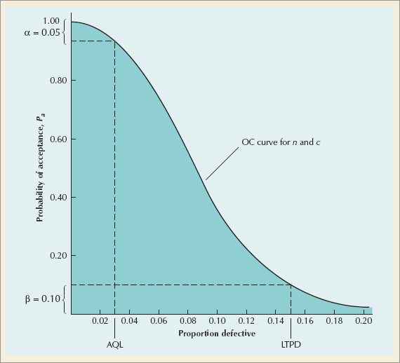
The performance measures we described in the previous section for a sampling plan can be represented graphically with an operating characteristic (OC) curve. The OC curve measures the probability of accepting a lot for different quality (proportion defective) levels given a specific sample size (n) and acceptance level (c). Management can use such a graph to determine if their sampling plan meets the performance measures they have established for AQL, LTPD, α, and β. Thus, the OC curve indicates to management how effective the sampling plan is in distinguishing (more commonly known as discriminating) between good and bad lots. The shape of a typical OC curve for a single-sample plan is shown in Figure S3.1 on the next page.
In Figure S3.1 the percentage defective in a lot is shown along the horizontal axis, whereas the probability of accepting a lot is measured along the vertical axis. The exact shape and location of the curve is defined by the sample size (n) and acceptance level (c) for the sampling plan.
In Figure S3.1, if a lot has 3% defective items, the probability of accepting the lot (based on the sampling plan defined by the OC curve) is 0.95. If management defines the AQL as 3%, then the probability that an acceptable lot will be rejected (α) is 1 minus the probability of accepting a lot or 1 – 0.95 = 0.05. If management is willing to accept lots with a percentage defective up to 15% (i.e., the LTPD), this corresponds to a probability that the lot will be accepted (β) of 0.10. A frequently used set of performance measures is α = 0.05 and β = 0.10.
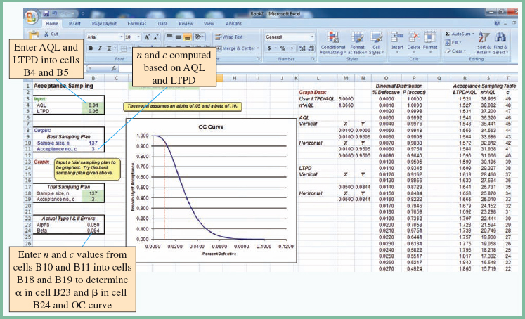
Developing a sampling plan manually requires a tedious trial-and-error approach using statistical analysis. n and c are progressively changed until an approximate sampling plan is obtained that meets the specified performance measures. A more practical alternative is to use OM Tools. Example S3.1 demonstrates the use of OM Tools to develop a sampling plan.
The shape of the operating characteristic curve shows that lots with a low percentage of defects have a high probability of being accepted, and lots with a high percentage of defects have a low probability of being accepted, as one would expect. For example, using the OC curve for the sampling plan in Example S3.1 (n = 137, c ≤ 3) for a percentage of defects = 0.01, the probability the lot will be accepted is approximately 0.95, whereas for 0.05, the probability of accepting a lot is relatively small. However, all lots, whether or not they are accepted, will pass on some defective items to the customer. The average outgoing quality (AOQ) is a measure of the expected number of defective items that will pass on to the customer with the sampling plan selected.
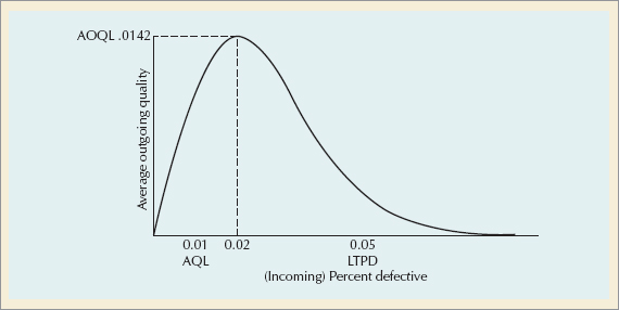
When a lot is rejected as a result of the sampling plan, it is assumed that it will be subjected to a complete inspection, and all defective items will be replaced with good ones. Also, even when a lot is accepted, the defective items found in the sample will be replaced. Thus, some portion of all the defective items contained in all the lots produced will be replaced before they are passed on to the customer. The remaining defective items that make their way to the customer are contained in lots that are accepted. Figure S3.2 shows the average outgoing quality curve for Example S3.1
The maximum point on the curve is referred to as the average outgoing quality limit (AOQL). For our example, the AOQL is 1.42% defective when the actual proportion defective of the lot is 2%. This is the worst level of outgoing quality that management can expect on average, and if this level is acceptable, then the sampling plan is deemed acceptable. Notice that as the percentage of defects increases and the quality of the lots deteriorates, the AOQ improves. This occurs because as the quality of the lots becomes poorer, it is more likely that bad lots will be identified and rejected, and any defective items in these lots will be replaced with good ones.
•Average outgoing quality (AOQ): the expected number of defective items that will pass on to the customer with a sampling plan.
In a double-sampling plan, a small sample is taken first; if the quality is very good, the lot is accepted, and if the sample is very poor, the lot is rejected. However, if the initial sample is inconclusive, a second sample is taken and the lot is either accepted or rejected based on the combined results of the two samples. The objective of such a sampling procedure is to save costs relative to a single-sampling plan. For very good or very bad lots, the smaller, less expensive sample will suffice and a larger, more expensive sample is avoided.
Double-sampling plans are less costly than single-sampling plans.
A multiple-sampling plan, also referred to as a sequential-sampling plan, generally employs the smallest sample size of any of the sampling plans we have discussed. In its most extreme form, individual items are inspected sequentially, and the decision to accept or reject a lot is based on the cumulative number of defective items. A multiple-sampling plan can result in small samples and, consequently, can be the least expensive of the sampling plans.
A multiple-sampling plan uses the smallest sample size of any sampling plan.
The steps of a multiple-sampling plan are similar to those for a double-sampling plan. An initial sample (which can be as small as one unit) is taken. If the number of defective items is less than or equal to a lower limit, the lot is accepted, whereas if it exceeds a specifid upper limit, the lot is rejected. If the number of defective items falls between the two limits, a second sample is obtained. The cumulative number of defects is then compared with an increased set of upper and lower limits, and the decision rule used in the first sample is applied. If the lot is neither accepted nor rejected with the second sample, a third sample is taken, with the acceptance/rejection limits revised upward. These steps are repeated for subsequent samples until the lot is either accepted or rejected.
Choosing among single-, double-, or multiple-sampling plans is an economic decision. When the cost of obtaining a sample is very high compared with the inspection cost, a single-sampling plan is preferred. For example, if a petroleum company is analyzing soil samples from various locales around the globe, it is probably more economical to take a single, large sample in Brazil than to return for additional samples if the initial sample is inconclusive. Alternatively, if the cost of sampling is low relative to inspection costs, a double- or multiple-sampling plan may be preferred. For example, if a winery is sampling bottles of wine, it may be more economical to use a sequential sampling plan, tasting individual bottles, than to test a large single sample containing a number of bottles, since each bottle sampled is, in effect, destroyed. In most cases in which quality control requires destructive testing, the inspection costs are high compared with sampling costs.
Four decades ago acceptance sampling constituted the primary means of quality control in many U.S. companies. However, it is the exception now, as most quality-conscious firms in the United States and abroad have either adopted or moved toward a quality-management program such as a OMS or Six Sigma. The cost of inspection, the cost of sending lots back, and the cost of scrap and waste are costs that most companies cannot tolerate and remain competitive in today's global market. Still, acceptance sampling is used by some companies and government agencies, and thus it is a relevant topic for study.
acceptable quality level (AQL) the fraction of defective items deemed acceptable in a lot.
acceptance sampling a statistical procedure for taking a random sample in order to determine whether or not a lot should be accepted or rejected.
average outgoing quality (AOQ) the expected number of defective items that will pass on to the customer with a sampling plan.
consumer's risk (β) the profitability of accepting a lot in which the fraction of defective items exceeds the most (LTPD) the consumer is willing to accept.
lot tolerance percent defective (LTPD) the maximum percentage defective items in a lot that the consumer will knowingly accept.
operating characteristic (OC) curve a graph that measures the probability of accepting a lot for different proportions of defective items.
producer's risk (α) the probability of rejecting a lot that has an acceptable quality level (AQL).
sampling plan a plan that provides guidelines for accepting a lot.
SINGLE-SAMPLE, ATTRIBUTE PLAN
PROBLEM STATEMENT
A product lot of 2000 items is inspected at a station at the end of the production process. Management and the product's customer have agreed to a quality-control program whereby lots that contain no more than 2% defectives are deemed acceptable, whereas lots with 6% or more defectives are not acceptable. Furthermore, management desires to limit the probability that a good lot will be rejected to 5%, and the customer wants to limit the probability that a bad lot will be accepted to 10%. Using OM Tools, develop a sampling plan that will achieve the quality-performance criteria.
SOLUTION
The OM Tools solution is shown as follows:
S3-1. What is the difference between acceptance sampling and sampling and process control?
S3-2. Why are sample sizes for attributes necessarily larger than sample sizes for variables?
S3-3. How is the sample size determined in a single-sample attribute plan?
S3-4. How does the AQL relate to producer's risk (α) and the LTPD relate to consumer's risk (β)?
S3-5. Explain the difference between single-, double-, and multiple-sampling plans.
S3-6. Why is the traditional view of quality control reflected in the use of acceptance sampling unacceptable to adherents of quality management and continuous improvement.
S3-7 Under what circumstances is the total inspection of final products necessary?
S3-1. The Great Lakes Company, a grocery store chain, purchases apples from a produce distributor in Virginia. The grocery company has an agreement with the distributor that it desires shipments of 10,000 apples with no more than 2% defectives (i.e., severely blemished apples), although it will accept shipments with up to a maximum of 8% defective. The probability of rejecting a good lot is set at 0.05, whereas the probability of accepting a bad-quality lot is 0.10. Determine a sampling plan that will approximately achieve these quality performance criteria, and the operating characteristic curve.
S3-2. The Academic House Publishing Company sends out the textbooks it publishes to an independent book binder. When the bound books come back, they are inspected for defective bindings (e.g., warped boards, ripples, cuts, poor adhesion). The publishing company has an acceptable quality level of 4% defectives but will tolerate lots of up to 10% defective. What (approximate) sample size and acceptance level would result in a probability of 0.05 that a good lot will be rejected and a probability of 0.10 that a bad lot will be accepted?
S3-3. The Metro Packaging Company in Richmond produces clear plastic bottles for the Kooler Cola Company, a soft-drink manufacturer. Metro inspects each lot of 5000 bottles before they are shipped to the Kooler Company. The soft-drink company has specified an acceptable quality level of 0.06 and a lot tolerance percent defective of 0.12. Metro currently has a sampling plan with n = 150 and c ≤ 4. The two companies have recently agreed that the sampling plan should have a producer's risk of 0.05 and a consumer's risk of 0.10. Will the current sampling plan used by Metro achieve these levels of α and β?
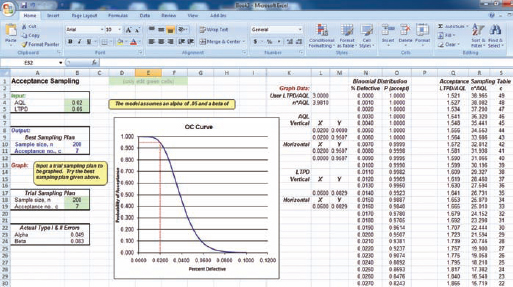
S3-4. The Fast Break Computer Company assembles personal computers and sells them to retail outlets. It purchases keyboards for its PCs from a manufacturer in the Orient. The keyboards are shipped in lots of 1000 units, and when they arrive at the Fast Break Company samples are inspected. Fast Break's contract with the overseas manufacturer specifies that the quality level that they will accept is 4% defective. The personal computer company wants to avoid sending a shipment back because the distance involved would delay and disrupt the assembly process; thus, they want only a 1% probability of sending a good lot back. The worst level of quality the Fast Break Company will accept is 10% defective items. Using OM Tools develop a sampling plan that will achieve these quality-performance criteria.
S3-5. A department store in Beijing, China, has arranged to purchase specially designed sweatshirts with the Olympic logo from a clothing manufacturer in Hong Kong. When the sweatshirts arrive in Beijing in lots of 2000 units, they are inspected. The store's management and manufacturer have agreed on quality criteria of AQL = 2% defective and LTPD = 8% defective. Because sending poor-quality shipments back to Hong Kong would disrupt sales at the stores, management has specified a low producer's risk of 0.01 and will accept a relatively high consumer's risk of 0.10. Using OM Tools, develop a sampling plan that will achieve these quality-performance criteria.