
In this chapter, you will learn about . . .
The Strategic Role of Forecasting in Supply Chain Management
Components of Forecasting Demand
Time Series Methods
Forecast Accuracy
Time Series Forecasting Using Excel
Regression Methods
Web resources for this chapter include
OM Tools Software
Animated Demo Problems
Internet Exercises
Online Practice Quizzes
Lecture Slides in PowerPoint
Virtual Tours
Excel Worksheets
Excel Exhibits
Company and Resource Weblinks
www.wiley.com/college/russell
Forecasting AT HERSHEY'S
Global companies like Hershey have numerous opportunities to use forecasting along various points in its supply chain. Downstream in its supply chain Hershey's attempts to forecast product demand, which is subject to uncertainties resulting from new and current products from competitors, competitors' promotional events and price changes, and changing consumer tastes for its own current and new products. Issues related to product quality and safety, ingredients, or packaging could adversely affect demand. Negative publicity related to product recalls due to contamination or product tampering, whether valid or not, might also negatively impact product demand. All of these factors affect the forecasting process. Upstream in its supply chain Hershey's sources many different commodities including cocoa products, sugar, dairy products, peanuts, almonds, corn sweeteners, natural gas, and fuel oil. Commodities are subject to price volatility and changes in supply can be caused by numerous factors, including commodity market fluctuations and speculative influences; currency exchange rates; the effect of weather on crop yield and distribution channels; trade agreements among producing and consuming nations; political unrest in producing countries; and changes in governmental agricultural programs and energy policies. Other factors that can create uncertainties in its global supply chain and operations that make forecasting difficult include global economic and environmental changes that can result in interruptions in supply and decreased demand for its products overseas; changes in tariff and trade agreements; political instability; nationalization of Hershey's properties; and disruptions in shipping or reduced availability of freight transportation.
In this chapter we will learn about the various forecasting methods and techniques that companies like Hershey's use to forecast demand for their products that drive the entire supply chain management process.
Source: The Hershey's Web site at www.thehersheycompany.com
A forecast is a prediction of what will occur in the future. Meteorologists forecast the weather, sportscasters and gamblers predict the winners of football games, and compa-nies attempt to predict how much of their product will be sold in the future. A forecast of product demand is the basis for most important planning decisions. Planning decisions regarding scheduling, inventory, production, facility layout and design, workforce, distribution, purchasing, and so on, are functions of customer demand. Long-range, strategic plans by top management are based on forecasts of the type of products consumers will demand in the future and the size and location of product markets.
Forecasting is an uncertain process. It is not possible to predict consistently what the future will be, even with the help of a crystal ball or a deck of tarot cards. Management generally hopes to forecast demand with as much accuracy as possible, which is becoming increasingly difficult to do. In the current international business environment, consumers have more product choices and more information on which to base choices. They also demand and receive greater product diversity, made possible by rapid technological advances. This makes forecasting products and product demand more difficult. Consumers and markets have never been stationary targets, but they are moving more rapidly now than they ever have before.
• Qualitative forecast methods: subjective methods.
• Quantitative forecast methods: are based on mathematical formulas.
Companies sometimes use qualitative forecast methods based on judgment, opinion, past experience, or best guesses, to make forecasts. A number of quantitative forecasting methods are also available to aid management in making planning decisions. In this chapter we discuss two of the traditional types of mathematical forecasting methods, time series analysis and regression, as well as several nonmathematical, qualitative approaches to forecasting. Although no technique will result in a totally accurate forecast, these methods can provide reliable guidelines in making decisions.
In today's global business environment, strategic planning and design tend to focus on supply chain management and quality management.
A company's supply chain encompasses all of the facilities, functions, and activities involved in producing a product or service from suppliers (and their suppliers) to customers (and their customers). Supply chain functions include purchasing, inventory, production, scheduling, facility location, transportation, and distribution. All these functions are affected in the short run by product demand and in the long run by new products and processes, technology advances, and changing markets.
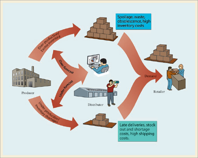
Forecasts of product demand determine how much inventory is needed, how much product to make, and how much material to purchase from suppliers to meet forecasted customer needs. This in turn determines the kind of transportation that will be needed and where plants, warehouses, and distribution centers will be located so that products and services can be delivered on time. Without accurate forecasts, large stocks of costly inventory must be kept at each stage of the supply chain to compensate for the uncertainties of customer demand. If there are insufficient inventories, customer service suffers because of late deliveries and stockouts. This is especially hurtful in today's competitive global business environment, where customer service and on-time delivery are critical factors. Figure 12.1 illustrates the effects of bad forecasting on the supply chain.
Accurate forecasting determines how much inventory a company must keep at various points along its supply chain.
While accurate forecasts are necessary, completely accurate forecasts are never possible. Hopefully, the forecast will reduce uncertainty about the future as much as possible, but it will never eliminate uncertainty. As such, all of the supply chain processes need to be flexible to respond to some degree of uncertainty.
In Chapter 10 on supply chain management, we talked about the "bullwhip effect" and its negative impact on the supply chain. The bullwhip effect is the distortion of information about product demand (including forecasts) as it is transmitted up the supply chain back toward suppliers. As demand moves further away from the ultimate end-use consumer, the variation in demand becomes greater and demand forecasts become less reliable. This increased variation can result in excessive, costly safety stock inventories at each stage in the supply chain and poorer customer service.
The bullwhip effect is caused when slight demand variability is magnified as information moves back upstream in the supply chain (see Figure 10.4). It is created when supply chain members make ordering decisions with an eye to their own self-interest and/or they do not have accurate demand forecasts from adjacent supply chain members. If each supply chain member is uncertain and not confident about what the actual demand is for the succeeding member it supplies, and it's making its own demand forecast, then it will stockpile extra inventory to compensate for the uncertainty; that is, the member creates a security blanket of inventory. One way to cope with the bullwhip effect is to develop demand forecasts that will reduce uncertainty and for supply chain members to share these forecasts with each other. Ideally, a single forecast of demand for the final customer in the supply chain would drive the development of subsequent forecasts for each supply chain member back up through the supply chain.
One trend in supply chain design is continuous replenishment, wherein continuous updating of data is shared between suppliers and customers. In this system, customers are continuously being replenished, daily or even more often, by their suppliers based on actual sales. Continuous replenishment, typically managed by the supplier, reduces inventory for the company and speeds customer delivery. Variations of continuous replenishment include quick response, just-in-time (JIT), VMI (vendor-managed inventory), and stockless inventory. Such systems rely heavily on accurate short-term forecasts, usually on a weekly basis, of end-use sales to the ultimate customer. The supplier at one end of a company's supply chain must forecast the company's customer demand at the other end of the supply chain in order to maintain continuous replenishment. The forecast also has to be able to respond to sudden, quick changes in demand. Longer forecasts based on historical sales data for 6 to 12 months into the future are also generally required to help make weekly forecasts and suggest trend changes.
In continuous replenishment, the supplier and customer share continuously updated data.
Forecasting is also crucial in a quality management environment. More and more, customers perceive good-quality service to mean having a product when they demand it. This holds true for manufacturing and service companies. When customers walk into a McDonald's to order a meal, they do not expect to wait long to place orders. They expect McDonald's to have the item they want, and they expect to receive their orders within a short period of time. A good forecast of customer traffic flow and product demand enables McDonald's to schedule enough servers, to stock enough food, and to schedule food production to provide high-quality service. An inaccurate forecast causes service to break down, resulting in poor quality. For manufacturing operations, especially for suppliers, customers expect parts to be provided when demanded. Accurately forecasting customer demand is a crucial part of providing the high-quality service.
Forecasting customer demand is a key to providing good-quality service.
There can be no strategic planning without forecasting. The ultimate objective of strategic planning is to determine what the company should be in the future—what markets to compete in, with what products, to be successful and grow. To answer these questions, the company needs to know what new products its customers will want, how much of these products customers will want, and the level of quality and other features that will be expected in these products. Forecasting answers these questions and is a key to a company's long-term competitiveness and success. The determination of future new products and their design subsequently determines process design, the kinds of new equipment and technologies that will be needed, and the design of the supply chain, including the facilities, transportation, and distribution systems that will be required. These elements are ultimately based on the company's forecast of the long-run future.
Successful strategic planning requires accurate forecasts of future products and markets.
The type of forecasting method depends on time frame, demand behavior, and causes of behavior.
The type of forecasting method to use depends on several factors, including the time frame of the Time frame of the forecast (i.e., how far in the future is being forecasted), the behavior of demand, and the possible existence of patterns (trends, seasonality, and so on), and the causes of demand behavior.
• Time frame: indicates how far into the future is forecast.
• Short- to mid-range forecast: typically encompasses the immediate future–daily up to two years.
Forecasts are either short- to mid-range, or long-range. Short-range (to mid-range) forecasts are typically for daily, weekly, or monthly sales demand for up to approximately two years into the future, depending on the company and the type of industry. They are primarily used to determine production and delivery schedules and to establish inventory levels. At Hewlett-Packard monthly forecasts for printers are constructed from 12 to 18 months into the future, while at Levi Strauss weekly forecasts for jeans are prepared for five years into the future.
• Long-range forecast: usually encompasses a period of time longer than two years.
A long-range forecast is usually for a period longer than two years into the future. A long-range forecast is normally used for strategic planning—to establish long-term goals, plan new products for changing markets, enter new markets, develop new facilities, develop technology, design the supply chain, and implement strategic programs. At Unisys, long-range strategic forecasts project three years into the future; Hewlett-Packard's long-term forecasts are developed for years 2 through 6; and at Fiat, the Italian automaker, strategic plans for new and continuing products go 10 years into the future.
These classifications are generalizations. The line between short- and long-range forecasts is not always distinct. For some companies a short-range forecast can be several years, and for other firms a long-range forecast can be in terms of months. The length of a forecast depends a lot on how rapidly the product market changes and how susceptible the market is to technological changes.
Demand sometimes behaves in a random, irregular way. At other times it exhibits predictable behavior, with trends or repetitive patterns, which the forecast may reflect. The three types of demand behavior are trends, cycles, and seasonal patterns.
• Trend: a gradual, long-term up or down movement of demand.
• Random variations: movements in demand that do not follow a pattern.
• Cycle: an up-and-down repetitivemovement in demand.
A trend is a gradual, long-term up or down movement of demand. For example, the demand for houses has followed an upward trend during the past few decades, without any sustained downward movement in the market. Trends are often the starting points for developing forecasts. Figure 12.2 (a) illustrates a demand trend in which there is a general upward movement, or increase. Notice that Figure 12.2(a) also includes several random movements up and down. Random variations are movements that are not predictable and follow no pattern (and thus are virtually unpredictable). They are routine variations that have no "assignable" cause.
A cycle is an up-and-down movement in demand that repeats itself over a lengthy time span (i.e., more than a year). For example, new housing starts and, thus, construction-related products tend to follow cycles in the economy. Automobile sales also tend to follow cycles. The demand for winter sports equipment increases every four years before and after the Winter Olympics. Fig-ure 12.2(b) shows the behavior of a demand cycle.
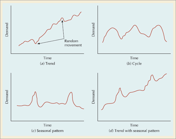
A seasonal pattern is an oscillating movement in demand that occurs periodically (in the short run) and is repetitive. Seasonality is often weather-related. For example, every winter the demand for snowblowers and skis increases, and retail sales in general increase during the holiday season. However, a seasonal pattern can occur on a daily or weekly basis. For example, some restaurants are busier at lunch than at dinner, and shopping mall stores and theaters tend to have higher demand on weekends. At FedEx seasonalities include the month of the year, day of the week, and day of the month, as well as various holidays. Figure 12.2c illustrates a seasonal pattern in which the same demand behavior is repeated each year at the same time.
• Seasonal pattern: an up-and-down repetitive movement in demand occurring periodically.
Demand behavior frequently displays several of these characteristics simultaneously. Although housing starts display cyclical behavior, there has been an upward trend in new house construction over the years. Demand for skis is seasonal; however, there has been an upward trend in the demand for winter sports equipment during the past two decades. Figure 12.2d displays the combination of two demand patterns, a trend with a seasonal pattern.
Instances when demand behavior exhibits no pattern are referred to as irregular movements, or variations. For example, a local flood might cause a momentary increase in carpet demand, or a competitor's promotional campaign might cause a company's product demand to drop for a time. Although this behavior has a cause and, thus, is not totally random, it still does not follow a pattern that can be reflected in a forecast.
The factors discussed previously in this section determine to a certain extent the type of forecasting method that can or should be used. In this chapter we are going to discuss three basic types of forecasting: time series methods, regression methods, and qualitative methods.
Types of methods: time series, causal, and qualitative.
Time series methods are statistical techniques that use historical demand data to predict future demand. Regression (or causal) forecasting methods attempt to develop a mathematical relationship (in the form of a regression model) between demand and factors that cause it to behave the way it does. Most of the remainder of this chapter will be about time series and regression forecasting methods. In this section we will focus our discussion on qualitative forecasting.
• Regression forecasting methods: relate demand to other factors that cause demand behavior.
Qualitative (or judgmental) methods use management judgment, expertise, and opinion to make forecasts. Often called "the jury of executive opinion," they are the most common type of forecasting method for the long-term strategic planning process. There are normally individuals or groups within an organization whose judgments and opinions regarding the future are as valid or more valid than those of outside experts or other structured approaches. Top managers are the key group involved in the development of forecasts for strategic plans. They are generally most familiar with their firms' own capabilities and resources and the markets for their products.
Management, marketing and purchasing, and engineering are sources for internal qualitative forecasts.
The sales force of a company represents a direct point of contact with the consumer. This contact provides an awareness of consumer expectations in the future that others may not possess. Engineering personnel have an innate understanding of the technological aspects of the type of products that might be feasible and likely in the future.
Consumer, or market, research is an organized approach using surveys and other research techniques to determine what products and services customers want and will purchase, and to identify new markets and sources of customers. Consumer and market research is normally conducted by the marketing department within an organization, by industry organizations and groups, and by private marketing or consulting firms. Although market research can provide accurate and useful forecasts of product demand, it must be skillfully and correctly conducted, and it can be expensive.
• Delphi method: involves soliciting forecasts about technological advances from experts.
The Delphi method is a procedure for acquiring informed judgments and opinions from knowledgeable individuals using a series of questionnaires to develop a consensus forecast about what will occur in the future. It was developed at the Rand Corporation shortly after World War II to forecast the impact of a hypothetical nuclear attack on the United States. Although the Delphi method has been used for a variety of applications, forecasting has been one of its primary uses. It has been especially useful for forecasting technological change and advances.
Technological forecasting has become increasingly crucial to compete in the modern international business environment. New enhanced computer technology, new production methods, and advanced machinery and equipment are constantly being made available to companies. These advances enable them to introduce more new products into the marketplace faster than ever before. The companies that succeed manage to get a "technological" jump on their competitors by accurately predicting what technology will be available in the future and how it can be exploited. What new products and services will be technologically feasible, when they can be introduced, and what their demand will be are questions about the future for which answers cannot be predicted from historical data. Instead, the informed opinion and judgment of experts are necessary to make these types of single, long-term forecasts.
Forecasting is a continuous process.
Forecasting is not simply identifying and using a method to compute a numerical estimate of what demand will be in the future. It is a continuing process that requires constant monitoring and adjustment illustrated by the steps in Figure 12.3.
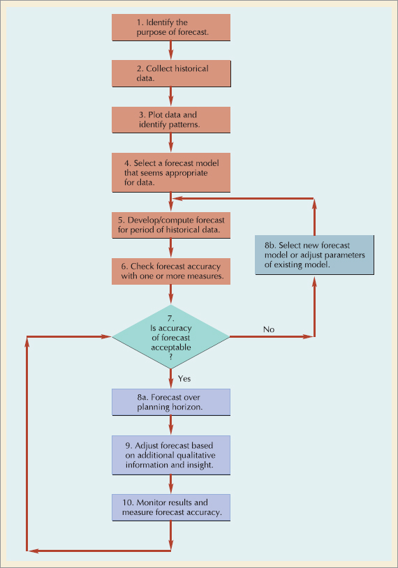
In the next few sections, we present several different forecasting methods applicable for different patterns of demand behavior. Thus, one of the first steps in the forecasting process is to plot the available historical demand data and, by visually looking at them, to attempt to determine the forecasting method that best seems to fit the patterns the data exhibit. Historical demand is usually past sales or orders data. There are several measures for comparing historical demand with the forecast to see how accurate the forecast is. Following our discussion of the forecasting methods, we present several measures of forecast accuracy. If the forecast does not seem to be accurate, another method can be tried until an accurate forecast method is identified. After the forecast is made over the desired planning horizon, it may be possible to use judgment, experience, knowl-edge of the market, or even intuition to adjust the forecast to enhance its accuracy. Finally, as demand actually occurs over the planning period, it must be monitored and compared with the forecast in order to assess the performance of the forecast method. If the forecast is accurate, then it is appropriate to continue using the forecast method. If it is not accurate, a new model or adjust-ing the existing one should be considered.
Time series methods are statistical techniques that make use of historical data accumulated over a period of time. Time series methods assume that what has occurred in the past will continue to occur in the future. As the name time series suggests, these methods relate the forecast to only one factor—time. These methods assume that identifiable historical patterns or trends for demand over time will repeat themselves. They include the moving average, exponential smoothing, and linear trend line; and they are among the most popular methods for short-range forecasting among service and manufacturing companies. In a 2007 survey of firms across different industries conducted by the Institute of Business Forecasting, over 60% of the firms used time series models, making it the most popular forecasting method by far. One of the reasons time series models are so popular is that they are relatively easy to understand and use. The survey also showed that the most popular time series models are moving averages and exponential smoothing.[17]
• Time series methods: use historical demand data over a period of time to predict future demand.
In a naive forecast demand in the current period is used as the next period's forecast.
A time series forecast can be as simple as using demand in the current period to predict demand in the next period. This is sometimes called a naive or intuitive forecast. For example, if demand is 100 units this week, the forecast for next week's demand is 100 units; if demand turns out to be 90 units instead, then the following week's demand is 90 units, and so on. This type of forecasting method does not take into account historical demand behavior; it relies only on demand in the current period. It reacts directly to the normal, random movements in demand.
• Moving average: method uses average demand for a fixed sequence of periods.
The simple moving average method uses several demand values during the recent past to develop a forecast. This tends to dampen, or smooth out, the random increases and decreases of a forecast that uses only one period. The simple moving average is useful for forecasting demand that is stable and does not display any pronounced demand behavior, such as a trend or seasonal pattern.
Moving average is good for stable demand with no pronounced behavioral patterns.
Moving averages are computed for specific periods, such as three months or five months, depending on how much the forecaster desires to "smooth" the demand data. The longer the moving average period, the smoother it will be. (Alternatively, a shorter moving average is more susceptible to simple random variation.) The formula for computing the simple moving average is

where
n = number of periods in the moving average
Di = demand in period i
Computing a Simple Moving Average
The Heartland Produce Company sells and delivers food produce to restaurants and catering services within a 100-mile radius of its warehouse. The food supply business is competitive, and the ability to deliver orders promptly is a factor in getting new customers and keeping old ones. The manager of the company wants to be certain enough drivers and vehicles are available to deliver orders promptly and they have adequate inventory in stock. Therefore, the manager wants to be able to forecast the number of orders that will occur during the next month (i.e., to forecast the demand for deliveries).
From records of delivery orders, management has accumulated the following data for the past 10 months, from which it wants to compute three- and five-month moving averages.
Month | Orders |
|---|---|
January | 120 |
February | 90 |
March | 100 |
April | 75 |
May | 110 |
June | 50 |
July | 75 |
August | 130 |
September | 110 |
October | 90 |
Solution
Let us assume that it is the end of October. The forecast resulting from either the three- or five-month moving average is typically for the next month in the sequence, which in this case is November. The moving average is computed from the demand for orders for the prior three months in the sequence according to the following formula:
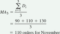
The five-month moving average is computed from the prior five months of demand data as follows:
The three- and five-month moving average forecasts for all the months of demand data are shown in the following table. Actually, the manager would use only the forecast for November based on the most recent monthly demand. However, the earlier forecasts for prior months allow us to compare the forecast with actual demand to see how accurate the forecasting method is—that is, how well it does.
Three- and Five-Month Averages
Month | Orders per Month | Three-Month Moving Average | Five-Month Moving Average |
|---|---|---|---|
January | 120 | — | — |
February | 90 | — | — |
March | 100 | — | — |
April | 75 | 103.3 | — |
May | 110 | 88.3 | — |
June | 50 | 95.0 | 99.0 |
July | 75 | 78.3 | 85.0 |
August | 130 | 78.3 | 82.0 |
September | 110 | 85.0 | 88.0 |
October | 90 | 105.0 | 95.0 |
November | — | 110.0 | 91.0 |
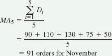
Both moving average forecasts in the preceding table tend to smooth out the variability occurring in the actual data. This smoothing effect can be observed in the following figure in which the three-month and five-month averages have been superimposed on a graph of the original data:
The five-month moving average in the previous figure smooths out fluctuations to a greater extent than the three-month moving average. However, the three-month average more closely reflects the most recent data available to the produce company manager. In general, forecasts using the longer-period moving average are slower to react to recent changes in demand than would those made using shorter-period moving averages. The extra periods of data dampen the speed with which the forecast responds. Establishing the appropriate number of periods to use in a moving average forecast often requires some amount of trial-and-error experimentation.
Longer-period moving averages react more slowly to recent demand changes than shorter-period moving averages; shorter-period moving averages are more susceptible to simple random variation.
The disadvantage of the moving average method is that it does not react to variations that occur for a reason, such as cycles and seasonal effects. Factors that cause changes are generally ignored. It is basically a "mechanical" method, which reflects historical data in a consistent way. However, the moving average method does have the advantage of being easy to use, quick, and relatively inexpensive. In general, this method can provide a good forecast for the short run, but it should not be pushed too far into the future.
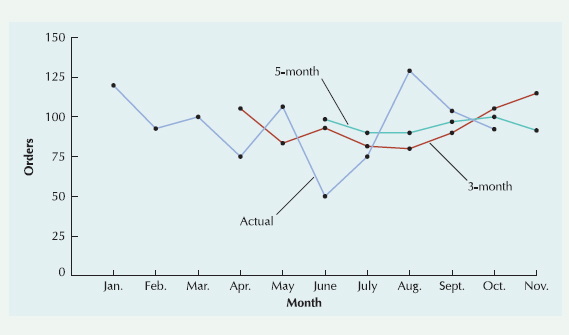
The moving average method can be adjusted to more closely reflect fluctuations in the data. In the weighted moving average method, weights are assigned to the most recent data according to the following formula:
where
Wi =the weight for period i, between 0 and 100 percent
Σ wi = 1.00
Determining the precise weights to use for each period of data usually requires some trial-and-error experimentation, as does determining the number of periods to include in the moving aver-age. If the most recent periods are weighted too heavily, the forecast might overreact to a random fluctuation in demand. If they are weighted too lightly, the forecast might underreact to actual changes in demand behavior.
Weighted moving average: weights are assigned to the most recent data.
Computing a Weighted Moving Average
The Heartland Produce Company in Example 12.1 wants to compute a three-month weighted moving average with a weight of 50% for the October data, a weight of 33% for the September data, and a weight of 17% for the August data. These weights reflect the company's desire to have the most recent data influence the forecast most strongly.
Solution
The weighted moving average is computed as
Notice that the forecast includes a fractional part, 0.4. In general, the fractional parts need to be included in the computation to achieve mathematical accuracy, but when the final forecast is achieved, it must be rounded up or down.
This forecast is slightly lower than our previously computed three-month average forecast of 110 orders, reflecting the lower number of orders in October (the most recent month in the sequence).
Exponential smoothing is also an averaging method that weights the most recent data more strongly. As such, the forecast will react more to recent changes in demand. This is useful if the recent changes in the data are significant and unpredictable instead of just random fluctuations (for which a simple moving average forecast would suffice).
• Exponential smoothing: an averaging method that reacts more strongly to recent changes in demand.
Exponential smoothing is one of the more popular and frequently used forecasting techniques, for a variety of reasons. Exponential smoothing requires minimal data. Only the forecast for the current period, the actual demand for the current period, and a weighting factor called a smoothing constant are necessary. The mathematics of the technique are easy to understand by management. Virtually all forecasting computer software packages include modules for exponential smoothing. Most importantly, exponential smoothing has a good track record of success. It has been employed over the years by many companies that have found it to be an accurate method of forecasting.
The exponential smoothing forecast is computed using the formula
where
Ft + 1 = the forecast for the next period
Dt = actual demand in the present period
Ft = the previously determined forecast for the present period
α = a weighting factor referred to as the smoothing constant
• Smoothing constant: the weighting factor given to the most recent data in exponential smoothing forecasts.
The smoothing constant, α, is between 0.0 and 1.0. It reflects the weight given to the most recent demand data. For example, if α = 0.20,
Ft+1 = 0.20Dt + 0.80Ft
which means that our forecast for the next period is based on 20% of recent demand (Dt) and 80% of past demand (in the form of forecast Ft, since Ft is derived from previous demands and fore-casts). If we go to one extreme and let α = 0.0, then
At many service-oriented businesses like fast food restaurants, quality service often equates with fast service. Taco Bell needs an accurate forecast of customer demand at different times during the day in order to provide fast, good quality service during peak demand periods around lunch and dinner.

and the forecast for the next period is the same as the forecast for this period. In other words, the forecast does not reflect the most recent demand at all.
On the other hand, if α = 1.0, then
The closer α is to 1.0, the greater the reaction to the most recent demand.
and we have considered only the most recent data (demand in the present period) and nothing else. Thus, the higher α is, the more sensitive the forecast will be to changes in recent demand, and the smoothing will be less. The closer α is to zero, the greater will be the dampening, or smoothing, effect. As α approaches zero, the forecast will react and adjust more slowly to differences between the actual demand and the forecasted demand. The most commonly used values of α are in the range of 0.01 to 0.50. However, the determination of α is usually judgmental and subjective and is often based on trial-and-error experimentation. An inaccurate estimate of α can limit the usefulness of this forecasting technique. (As α approaches 1.0, the forecast is the same as the naive result.)
Computing an ExponentiallySmoothed Forecast
HiTek Computer Services repairs and services personal computers at its store, and it makes local service calls. It primarily uses part-time State University students as technicians. The company has had steady growth since it started. It purchases generic computer parts in volume at a discount from a variety of sources whenever they see a good deal. Thus, they need a good forecast of demand for repairs so that they will know how many computer component parts to purchase and stock, and how many technicians to hire.
The company has accumulated the demand data shown in the accompanying table for repair and service calls for the past 12 months, from which it wants to consider exponential smoothing forecasts using smoothing constants (α) equal to 0.30 and 0.50.
Demand for Repair and Service Calls
Period | Month | Demand |
|---|---|---|
1 | January | 37 |
2 | February | 40 |
3 | March | 41 |
4 | April | 37 |
5 | May | 45 |
6 | June | 50 |
7 | July | 43 |
8 | August | 47 |
9 | September | 56 |
10 | October | 52 |
11 | November | 55 |
12 | December | 54 |
Solution
To develop the series of forecasts for the data in this table, we will start with period 1 (January) and compute the forecast for period 2 (February) using α = 0.30. The formula for exponential smoothing also requires a forecast for period 1, which we do not have, so we will use the demand for period 1 as both demand and forecast for period 1. (Other ways to determine a starting forecast include averaging the first three or four periods or making a subjective estimate.) Thus, the forecast for February is
The forecast for period 3 is computed similarly:
The remainder of the monthly forecasts are shown in the following table. The final forecast is for period 13, January, and is the forecast of interest to HiTek:
Exponential Smoothing Forecasts, α = 0.30 and α = 0.50
Period | Month | Demand | Forecast, Ft+1 | |
|---|---|---|---|---|
α = 0.30 | α = 0.50 | |||
1 | January | 37 | — | — |
2 | February | 40 | 37.00 | 37.00 |
3 | March | 41 | 37.90 | 38.50 |
4 | April | 37 | 38.83 | 39.75 |
5 | May | 45 | 38.28 | 38.37 |
6 | June | 50 | 40.29 | 41.68 |
7 | July | 43 | 43.20 | 45.84 |
8 | August | 47 | 43.14 | 44.42 |
10 | October | 52 | 47.81 | 50.85 |
11 | November | 55 | 49.06 | 51.42 |
12 | December | 54 | 50.84 | 53.21 |
13 | January | — | 51.79 | 53.61 |
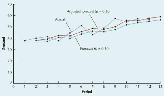
This table also includes the forecast values using α = 0.50. Both exponential smoothing forecasts are shown in the following figure together with the actual data.
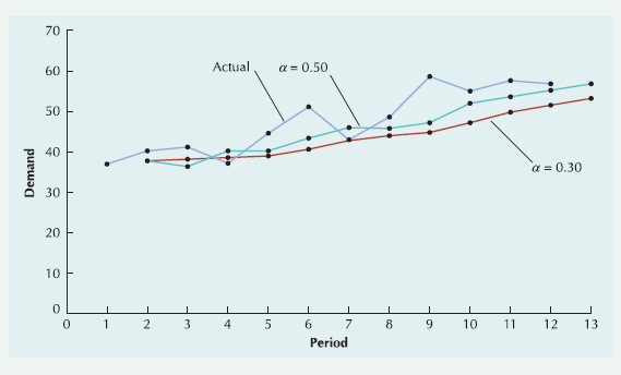
In Example 12.3, the forecast using the higher smoothing constant, α = 0.50, seems to react more strongly to changes in demand than does the forecast with α = 0.30, although both smooth out the random fluctuations in the forecast. Notice that both forecasts lag behind the actual demand. For example, a pronounced downward change in demand in July is not reflected in the forecast until August. If these changes mark a change in trend (i.e., a long-term upward or downward movement) rather than just a random fluctuation, then the forecast will always lag behind this trend. We can see a general upward trend in service calls throughout the year. Both forecasts tend to be consistently lower than the actual demand; that is, the forecasts lag the trend.
Based on simple observation of the two forecasts in Example 12.3, α = 0.50 seems to be the more accurate of the two in the sense that it seems to follow the actual data more closely. (Later in this chapter we discuss several quantitative methods for determining forecast accuracy.) When demand is relatively stable without any trend, a small value for α is more appropriate to simply smooth out the forecast. When actual demand displays an increasing (or decreasing) trend, as is the case in the figure, a larger value of α is better. It will react more quickly to more recent upward or downward movements in the actual data. In some approaches to exponential smoothing, the accuracy of the forecast is monitored in terms of the difference between the actual values and the forecasted values. If these differences become larger, then α is changed (higher or lower) in an attempt to adapt the forecast to the actual data. However, the exponential smoothing forecast can also be adjusted for the effects of a trend.
In Example 12.3, the final forecast computed was for one month, January. A forecast for two or three months could have been computed by grouping the demand data into the required number of periods and then using these values in the exponential smoothing computations. For example, if a three-month forecast were needed, demand for January, February, and March could be summed and used to compute the average forecast for the next three-month period, and so on, until a final three-month forecast results. Alternatively, if a trend is present, the final period forecast can be used for an extended forecast by adjusting it by a trend factor.
The adjusted exponential smoothing forecast consists of the exponential smoothing forecast with a trend adjustment factor added to it:
• Adjusted exponential smoothing forecast: an exponential smoothing forecast with an adjustment for a trend added to it.
where
T = an exponentially smoothed trend factor
The trend factor is computed much the same as the exponentially smoothed forecast. It is, in effect, a forecast model for trend:
where
Tt = the last period's trend factor
β = a smoothing constant for trend
The closer β is to 1.0 the stronger the trend is reflected.
β is a value between 0.0 and 1.0. It reflects the weight given to the most recent trend data. β is usually determined subjectively based on the judgment of the forecaster. A high β reflects trend changes more than a low β. It is not uncommon for β to equal α in this method.
Notice that this formula for the trend factor reflects a weighted measure of the increase (or decrease) between the next period forecast, Ft + 1, and the current forecast, Ft.
Computing an Adjusted Exponentially Smoothed Forecast
HiTek Computer Services now wants to develop an adjusted exponentially smoothed forecas using the same 12 months of demand shown in the table for Example 12.3. It will use the exponentially smoothed forecast with α = 0.5 computed in Example 12.3 with a smoothing constant for trend, β, of 0.30.
Solution
The formula for the adjusted exponential smoothing forecast requires an initial value for Tt to start the computational process. This initial trend factor is often an estimate determined subjectively or based on past data by the forecaster. In this case, since we have a long sequence of demand data (i.e., 12 months) we will start with the trend Tt equal to zero. By the time the forecast value of interest F13 is computed, we should have a relatively good value for the trend factor.
The adjusted forecast for February, AF2, is the same as the exponentially smoothed forecast, since the trend computing factor will be zero (i.e., F1 and F2 are the same and T2 = 0). Thus, we compute the adjusted forecast for March, AF3, as follows, starting with the determination of the trend factor, T3:
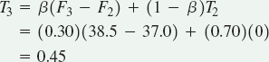
and
This adjusted forecast value for period 3 is shown in the accompanying table, with all other adjusted forecast values for the 12-month period plus the forecast for period 13, computed as follows:
and
Adjusted Exponential Smoothing Forecast Values
Period | Month | Demand | Forecast Ft + 1 | Trend Tt+1 | Adjusted Forecast AFt+1 |
|---|---|---|---|---|---|
1 | January | 37 | 37.00 | — | — |
2 | February | 40 | 37.00 | 0.00 | 37.00 |
3 | March | 41 | 38.50 | 0.45 | 38.95 |
4 | April | 37 | 39.75 | 0.69 | 40.44 |
5 | May | 45 | 38.37 | 0.07 | 38.44 |
6 | June | 50 | 41.68 | 1.04 | 42.73 |
7 | July | 43 | 45.84 | 1.97 | 47.82 |
8 | August | 47 | 44.42 | 0.95 | 45.37 |
9 | September | 56 | 45.71 | 1.05 | 46.76 |
10 | October | 52 | 50.85 | 2.28 | 53.13 |
11 | November | 55 | 51.42 | 1.76 | 53.19 |
12 | December | 54 | 53.21 | 1.77 | 54.98 |
13 | January | — | 53.61 | 1.36 | 54.96 |
The adjusted exponentially smoothed forecast values shown in the above table are compared with the exponentially smoothed forecast values and the actual data in the figure on the following page. Notice that the adjusted forecast is consistently higher than the exponentially smoothed forecast and is thus more reflective of the generally increasing trend of the actual data. However, in general, the pattern, or degree of smoothing, is very similar for both forecasts.
Linear regression is a method of forecasting in which a mathematical relationship is developed between demand and some other factor that causes demand behavior. However, when demand displays an obvious trend over time, a least squares regression line, or linear trend line, that relates demand to time, can be used to forecast demand.
• Linear trend line: a linear regression model relating demand to time.
A linear trend line relates a dependent variable, which for our purposes is demand, to one in-dependent variable, time, in the form of a linear equation:
y = a + bx
where
a = intercept (at period 0)
b = slope of the line
x = the time period
y = forecast for demand for period x
These parameters of the linear trend line can be calculated using the least squares formulas for linear regression:

where
Computing a Linear Trend Line
The data for HiTek Computer Services (shown in the table for Example 12.3) appears to follow an increasing linear trend. The company wants to compute a linear trend line to see if it is more accurate than the exponential smoothing and adjusted exponential smoothing forecasts developed in Examples 12.3 and 12.4.
Solution
The values required for the least squares calculations are as follows:
Least Squares Calculations
x (period) | y (demand) | xy | x2 |
|---|---|---|---|
1 | 37 | 37 | 1 |
2 | 40 | 80 | 4 |
3 | 41 | 123 | 9 |
4 | 37 | 148 | 16 |
5 | 45 | 225 | 25 |
6 | 50 | 300 | 36 |
7 | 43 | 301 | 49 |
8 | 47 | 376 | 64 |
9 | 56 | 504 | 81 |
10 | 52 | 520 | 100 |
11 | 55 | 605 | 121 |
12 | 54 | 648 | 144 |
78 | 557 | 3867 | 650 |
Using these values, we can compute the parameters for the linear trend line as follows:
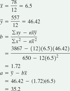
Therefore, the linear trend line equation is
y =35.2 +1.72x
To calculate a forecast for period 13, let x = 13 in the linear trend line:
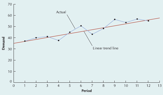
The graph on the following page shows the linear trend line compared with the actual data. The trend line appears to reflect closely the actual data—that is, to be a good fit—and would thus be a good forecast model for this problem. However, a disadvantage of the linear trend line is that it will not adjust to a change in the trend, as the exponential smoothing forecast methods will; that is, it is assumed that all future forecasts will follow a straight line. This limits the use of this method to a shorter time frame in which you can be relatively certain that the trend will not change.
A seasonal pattern is a repetitive increase and decrease in demand. Many demand items exhibit seasonal behavior. Clothing sales follow annual seasonal patterns, with demand for warm clothes increasing in the fall and winter and declining in the spring and summer as the demand for cooler clothing increases. Demand for many retail items, including toys, sports equipment, clothing, electronic appliances, hams, turkeys, wine, and fruit, increase during the holiday season. Greeting card demand increases in conjunction with special days such as Valentine's Day and Mother's Day. Seasonal patterns can also occur on a monthly, weekly, or even daily basis. Some restaurants have higher demand in the evening than at lunch or on weekends as opposed to weekdays. Traffic—hence sales—at shopping malls picks up on Friday and Saturday.

Snow skiing is an industry that exhibits several different patterns of demand behavior. It is primarily a seasonal (i.e., winter) industry and over a long period of time the snow skiing industry has exhibited a generally increasing growth trend. Random factors can cause variations, or abrupt peaks and valleys, in demand. For example, demand for skiing products always show a pronounced increase after the Winter Olympics.
• Seasonal factor: adjust for seasonality by multiplying the normal forecast by a seasonal factor.
There are several methods for reflecting seasonal patterns in a time series forecast. We will describe one of the simpler methods using a seasonal factor. A seasonal factor is a numerical value that is multiplied by the normal forecast to get a seasonally adjusted forecast.
One method for developing a demand for seasonal factors is to divide the demand for each seasonal period by total annual demand, according to the following formula:
The resulting seasonal factors between 0 and 1.0 are, in effect, the portion of total annual demand assigned to each season. These seasonal factors are multiplied by the annual forecasted demand to yield adjusted forecasts for each season.
Computing a Forecast with Seasonal Adjustments
Wishbone Farms grows turkeys to sell to a meat-processing company throughout the year. However, its peak season is obviously during the fourth quarter of the year, from October to December. Wishbone Farms has experienced the demand for turkeys for the past three years shown in the following table:
Demand for Turkeys at Wishbone Farms
Year | Demand (1000s) per Quarter | ||||
|---|---|---|---|---|---|
1 | 2 | 3 | 4 | Total | |
2008 | 12.6 | 8.6 | 6.3 | 17.5 | 45.0 |
2009 | 14.1 | 10.3 | 7.5 | 18.2 | 50.1 |
2010 | 15.3 | 10.6 | 8.1 | 19.6 | 53.6 |
Total | 42.0 | 29.5 | 21.9 | 55.3 | 148.7 |
Solution
Because we have three years of demand data, we can compute the seasonal factors by dividing total quarterly demand for the three years by total demand across all three years:
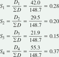
Next, we want to multiply the forecasted demand for the next year, 2008, by each of the seasonal factors to get the forecasted demand for each quarter. To accomplish this, we need a demand forecast for 2011. In this case, since the demand data in the table seem to exhibit a generally increasing trend, we compute a linear trend line for the three years of data in the table to get a rough forecast estimate:
Thus, the forecast for 2011 is 58.17, or 58,170 turkeys.
Using this annual forecast of demand, we find that the seasonally adjusted forecasts, SFi, for 2011 are
Comparing these quarterly forecasts with the actual demand values in the table, we see that they would seem to be relatively good forecast estimates, reflecting both the seasonal variations in the data and the general upward trend.
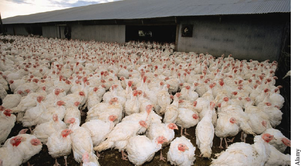
Turkeys are an example of a product with a long-term trend for increasing demand with a seasonal pattern. Turkey sales show a distinct seasonal pattern by increasing markedly during the Thanksgiving holiday season. For example, turkey sales are lowest from January to May, they begin to rise in June and July and peak in August when distributors begin to build up their inventory of frozen turkeys for increased sales in November. Sales remain high for September, October, and November and then begin to decline in December and January.
A forecast is never completely accurate; forecasts will always deviate from the actual demand. This difference between the forecast and the actual is the forecast error. Although forecast error is inevitable, the objective of forecasting is that it be as slight as possible. A large degree of error may indicate that either the forecasting technique is the wrong one or it needs to be adjusted by changing its parameters (for example, in the exponential smoothing forecast).
• Forecast error: the difference between the forecast and actual demand.
There are different measures of forecast error. We will discuss several of the more popular ones: mean absolute deviation (MAD), mean absolute percent deviation (MAPD), cumulative error, and average error or bias (Ē).
The mean absolute deviation, or MAD, is one of the most popular and simplest to use measures of forecast error. MAD is an average of the difference between the forecast and actual demand, as computed by the following formula:
• mean absolute deviation (MAD): the average, absolute difference between the forecast and demand.
where
t = the period number
Dt = demand in period t
Ft = the forecast for period t
n = the total number of periods
|| = absolute value
Measuring Forecasting Accuracy with MAD
In Examples 12.3, 12.4, and 12.5, forecasts were developed using exponential smoothing, (α = 0.30 and α = 0.50), adjusted exponential smoothing (α = 0.50, β = 0.30), and a linear trend line, respectively, for the demand data for HiTek Computer Services. The company wants to compare the accuracy of these different forecasts using MAD.
Solution
We will compute MAD for all four forecasts; however, we will present the computational detail for the exponential smoothing forecast with α = 0.30 only. The following table shows the values necessary to compute MAD for the exponential smoothing forecast:
Computational Values for MAD
Period | Demand, Dt | Forecast Ft (αi = 0.30) | Error (et) (Dt – Fi) | Dt – Ft |
|---|---|---|---|---|
1 | 37 | 37.00 | — | — |
2 | 40 | 37.00 | 3.00 | 3.00 |
3 | 41 | 37.90 | 3.10 | 3.10 |
4 | 37 | 38.83 | −1.83 | 1.83 |
5 | 45 | 38.28 | 6.72 | 6.72 |
6 | 50 | 40.29 | 9.69 | 9.69 |
7 | 43 | 43.20 | −0.20 | 0.20 |
8 | 47 | 43.14 | 3.86 | 3.86 |
9 | 56 | 44.30 | 11.70 | 11.70 |
10 | 52 | 47.81 | 4.19 | 4.19 |
11 | 55 | 49.06 | 5.94 | 5.94 |
12 | 54 | 50.84 | 3.15 | 3.15 |
557 | 49.32 | 53.38 |
The computation of MAD will be based on 11 periods, periods 2 through 12, excluding the initial demand and forecast values for period 1 since they both equal 37.
Using the data in the table, MAD is computed as
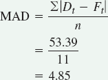
The smaller the value of MAD, the more accurate the forecast, although viewed alone, MAD is difficult to assess. In this example, the data values were relatively small, and the MAD value of 4.85 should be judged accordingly. Overall, it would seem to be a "low" value; that is, the forecast appears to be relatively accurate. However, if the magnitude of the data values were in the thousands or millions, then a MAD value of a similar magnitude might not be bad either. The point is, you cannot compare a MAD value of 4.85 with a MAD value of 485 and say the former is good and the latter is bad; they depend to a certain extent on the relative magnitude of the data.
The lower the value of MAD, relative to the magnitude of the data, the more accurate the forecast.
One benefit of MAD is to compare the accuracy of several different forecasting techniques, as we are doing in this example. The MAD values for the remaining forecasts are as follows:
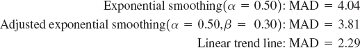
Since the linear trend line has the lowest MAD value of 2.29, it would seem to be the most accurate, although it does not appear to be significantly better than the adjusted exponential smoothing forecast. Furthermore, we can deduce from these MAD values that increasing α from 0.30 to 0.50 enhanced the accuracy of the exponentially smoothed forecast. The adjusted forecast is even more accurate.
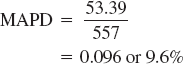
The mean absolute percent deviation (MAPD) measures the absolute error as a percentage of demand rather than per period. As a result, it eliminates the problem of interpreting the measure of accuracy relative to the magnitude of the demand and forecast values, as MAD does. The mean absolute percent deviation is computed according to the following formula:
• mean absolute percent deviation (MAPD): the absolute error as a percentage of demand.
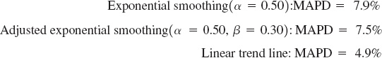
Using the data from the table in Example 12.7 for the exponential smoothing forecast (α = 0.30) for HiTek Computer Services,
A lower percent deviation implies a more accurate forecast. The MAPD values for our other three forecasts are
Cumulative error is computed simply by summing the forecast errors, as shown in the following formula.
• Cumulative error: the sum of the forecast errors.
A large positive value indicates that the forecast is probably consistently lower than the actual demand, or is biased low. A large negative value implies that the forecast is consistently higher than actual demand, or is biased high. Also, when the errors for each period are scrutinized, a preponderance of positive values shows the forecast is consistently less than the actual value and vice versa.
The cumulative error for the exponential smoothing forecast (α = 0.30) for HiTek Computer Services can be read directly from the table in Example 12.7; it is simply the sum of the values in the "Error" column:
Large +E indicates forecast is biased low; large −E, forecast is biased high.
This large positive error for cumulative error, plus the fact that the individual errors for all but two of the periods in the table are positive, indicates that this forecast is consistently below the actual demand. A quick glance back at the plot of the exponential smoothing (α = 0.30) forecast in Example 12.3 visually verifies this result.
The cumulative error for the other forecasts are
Exponential smoothing(α = 0.50): E = 33.21
Adjusted exponential smoothing(α = 0.50, β = 0.30): E = 21.14
We did not show the cumulative error for the linear trend line. E will always be near zero for the linear trend line.
A measure closely related to cumulative error is the average error, or bias. It is computed by averaging the cumulative error over the number of time periods:
• Average error: the per-period average of cumulative error.
For example, the average error for the exponential smoothing forecast (α = 0.30) is computed as follows. (Notice a value of 11 was used for n, since we used actual demand for the first-period forecast, resulting in no error, that is, D1 = F1 = 37.)
The average error is interpreted similarly to the cumulative error. A positive value indicates low bias, and a negative value indicates high bias. A value close to zero implies a lack of bias.
Table 12.1 summarizes the measures of forecast accuracy we have discussed in this section for the four example forecasts we developed in Examples 12.3, 12.4, and 12.5 for HiTek Computer Services. The results are consistent for all four forecasts, indicating that for the HiTek Computer Services example data, a larger value of is preferable for the exponential smoothing forecast. The adjusted forecast is more accurate than the exponential smoothing forecasts, and the linear trend is more accurate than all the others. Although these results are for specific examples, they indicate how the different forecast measures for accuracy can be used to adjust a forecasting method or select the best method.
There are several ways to monitor forecast error over time to make sure that the forecast is performing correctly—that is, the forecast is in control. Forecasts can go "out of control" and start providing inaccurate forecasts for several reasons, including a change in trend, the unanticipated appearance of a cycle, or an irregular variation such as unseasonable weather, a promotional campaign, new competition, or a political event that distracts consumers.
A tracking signal indicates if the forecast is consistently biased high or low. It is computed by dividing the cumulative error by MAD, according to the formula
• Tracking signal: monitors the forecast to see if it is biased high or low.
The tracking signal is recomputed each period, with updated, "running" values of cumulative error and MAD. The movement of the tracking signal is compared to control limits; as long as the tracking signal is within these limits, the forecast is in control.
Typically, forecast errors are normally distributed, which results in the following relationship between MAD and the standard deviation of the distribution of error, σ:
This enables us to establish statistical control limits for the tracking signal that corresponds to the more familiar normal distribution. For example, statistical control limits of ±3 standard deviations, corresponding to 99.7% of the errors, would translate to ±3.75 MADs; that is, 3σ ÷ 0.8 = 3.75 MADs. Control limits of ±2 to ±5 MADs are used most frequently.
Developing a Tracking Signal
In Example 12.7, the mean absolute deviation was computed for the exponential smoothing forecast (α = 0.30) for HiTek Computer Services. Using a tracking signal, monitor the forecast accuracy using control limits of ±3 MADs.
Solution
To use the tracking signal, we must recompute MAD each period as the cumulative error is computed.
Using MAD = 3.00, we find that the tracking signal for period 2 is
The tracking signal for period 3 is
The remaining tracking signal values are shown in the following table:
Tracking Signal Values
Period | Demand,Dt | Forecast,Ft | Error,Dt-Fi | E = Σ(Dt-Fi) | MAD | Tracking Signal |
|---|---|---|---|---|---|---|
1 | 37 | 37.00 | — | — | — | — |
2 | 40 | 37.00 | 3.00 | 3.00 | 3.00 | 1.00 |
3 | 41 | 37.90 | 3.10 | 6.10 | 3.05 | 2.00 |
4 | 37 | 38.83 | −1.83 | 4.27 | 2.64 | 1.62 |
5 | 45 | 38.28 | 6.72 | 10.99 | 3.66 | 3.00 |
6 | 50 | 40.29 | 9.69 | 20.68 | 4.87 | 4.25 |
7 | 43 | 43.20 | −0.20 | 20.48 | 4.09 | 5.01 |
8 | 47 | 43.14 | 3.86 | 24.34 | 4.06 | 6.00 |
9 | 56 | 44.30 | 11.70 | 36.04 | 5.01 | 7.19 |
10 | 52 | 47.81 | 4.19 | 40.23 | 4.92 | 8.18 |
11 | 55 | 49.06 | 5.94 | 46.17 | 5.02 | 9.20 |
12 | 54 | 50.84 | 3.15 | 49.32 | 4.85 | 10.17 |
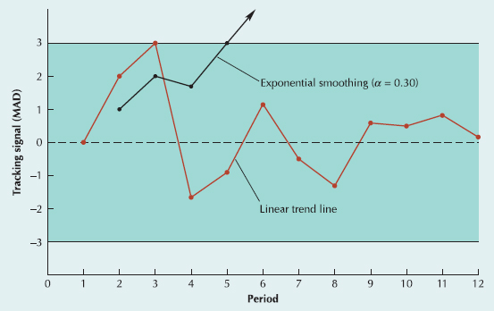
The tracking signal values in the table above move outside ±3 MAD control limits (i.e., ±3.00) in period 5 and continue increasing. This suggests that the forecast is not performing accurately or, more precisely, is consistently biased low (i.e., actual demand consistently exceeds the forecast). This is illustrated in the graph on the previous page. Notice that the tracking signal moves beyond the upper limit of 3 following period 5 and continues to rise. For the sake of comparison, the tracking signal for the linear trend line forecast computed in Example 12.5 is also plotted on this graph. Notice that it remains within the limits (touching the upper limit in period 3), indicating a lack of consistent bias.
Another method for monitoring forecast error is statistical control charts. For example, ±3σ control limits would reflect 99.7% of the forecast errors (assuming they are normally distributed). The sample standard deviation, σ, is computed as
This formula without the square root is known as the mean squared error (MSE), and it is sometimes used as a measure of forecast error. It reacts to forecast error much like MAD does. (For our Example 12.8, MSE = 37.57.)
• Mean squared error (MSE): the average of the squared forecast errors.
Forecast Error with Statistical Control Charts
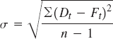
Using the same example for the exponential smoothing forecast (α = 0.30) for HiTek Computer Services, as in Example 12.8, we compute the standard deviation as
Using this value of σ we can compute statistical control limits for forecast errors for our exponential smoothing forecast (α = 0.30) example for HiTek Computer Services. Plus or minus 3σ control limits, reflecting 99.7% of the forecast errors, gives ±3(6.13), or ±18.39. Although it can be observed from the table in Example 12.8 that all the error values are within the control limits, we can still detect that most of the errors are positive, indicating a low bias in the forecast estimates. This is illustrated in the following graph of the control chart with the errors plotted on it.
ALONG THE SUPPLY CHAIN
Forecasting Market Demand at NBC
NBC Universal, a subsidiary of General Electric Company, owns and operates the most profitable television network in the United States with revenues of over $14 billion. Over 60% of these revenues were generated by on-air advertising time on its television networks and stations. The major television networks announce their new programming schedules for the upcoming season (which starts in late September) in mid-May. NBC begins selling their advertising time very soon after the new schedule is announced in May, and 60 to 80% of their airtime inventory is sold in the following two- to three-week period (to approximately 400 advertisers), known as the upfront market. Immediately following the announcement of their new season schedule in May, NBC forecasts ratings and estimates market demand for their shows. The ratings forecasts are estimates of the number of people in several demographic groups who are expected to watch each airing of the shows in the schedule for the entire year, which are, in turn, based on such factors as a show's strength, historical time slot ratings, and the ratings performance of adjacent shows. Total market demand depends primarily on the strength of the economy and the expected performance of the network's schedule. Based on this ratings forecast and market demand, NBC develops pricing strategies and sets the prices for commercials on their shows.
Forecasting the upfront market has always been a challenging process for NBC. In the past the network used historical patterns, expert knowledge, and intuition to forecast demand; then later it used time-series forecasting models based on historical demand. However, these models were unsatisfactory because of the unique nature of NBC's demand population of advertisers. NBC ultimately developed a unique approach to forecasting its upfront market for demand, which includes a combination of the Delphi technique and a "grass roots" forecasting approach. The Delphi technique seeks to develop a consensus (or at least a compromise) forecast from among a group of experts, while a grass roots approach to forecasting asks the individuals closest to the final customer, such as salespeople about the customer's purchasing plans. In their forecasting approach NBC used its (over 100) account executives, who interact closely with the network's (over 400) advertisers, to build a knowledge base in order to estimate individual advertiser's demand, aggregate this demand into a total demand forecast, and then continuously and iteratively update demand estimates based on the account executives expertise. Previous forecasting methods resulted in forecast errors of 5 to 12%, whereas this new forecasting process resulted in a forecast error of only 2.8%, the most accurate forecast NBC had ever achieved for its upfront market.

NBC uses various methods to forecast television ratings that indicate the number of viewers in different demographic groups that will watch their shows, which the network then uses to establish pricing strategies for the shows' commercials it will charge advertisers for.
Why do you think NBC's forecasting approach was more effective than a traditional time series forecasting model based on historical demand?
Source: S. Bollapragada, S. Gupta, B. Hurwitz, P. Miles and R. Tyagi "NBC–Universal Uses a Novel Qualitative Forecasting Technique to Predict Advertising Demand," Interfaces, vol. 38, (2: March–April, 2008), pp. 103–111.
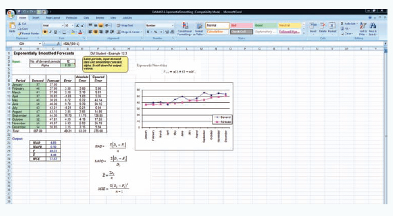
Excel can be used to develop forecasts using the moving average, exponential smoothing, ad-justed exponential smoothing, and linear trend line techniques. In a recent survey of companies across different industries that use forecasting, almost half use Excel spreadsheets for forecasting, while the rest use a variety of different forecasting software packages.[18]
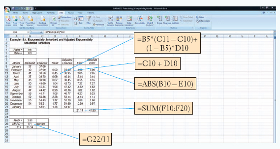
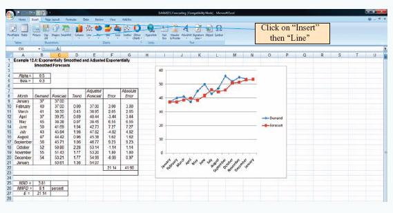
First we will demonstrate how to determine exponentially smoothed and adjusted exponen-tially smoothed forecasts using Excel, as shown in Exhibit 12.1. We will demonstrate Excel using Examples 12.3 and 12.4 for forecasting demand at HiTek Computer Services, including the Excel spreadsheets showing the exponentially smoothed forecast with α = 0.5 and the adjusted exponentially smoothed forecast with β = 0.3. We have also computed the values for MAD, MAPD, and E.
Notice that the formula in Exhibit 12.1 for computing the exponentially smoothed forecast for March is embedded in cell C11 and shown on the formula bar at the top of the screen. The same formula is used to compute all the other forecast values in column C. The formula for computing the trend value for March is B5*(C11 - C10) (1 - B5)*D10. The formula for the adjusted forecast in column E is computed by typing the formula C10 + D10 in cell E10 and copying it to cells E11:E21 (using the copy and paste options from the right mouse key). The error is computed for the adjusted forecast, and the formula for computing the error for March is B11 - E11, while the formula for absolute error for March is = ABS (F11).
A graph of the forecast can also be developed with Excel. To plot the exponentially smoothed forecast in column C and demand in column B, cover all cells from A8 to C21 with the mouse and click on "Insert" on the toolbar at the top of the worksheet. Next click on "Line," on the "Chart" toolbar. The resulting graph for demand and the exponentially smoothed forecast for our example is shown in Exhibit 12.2.
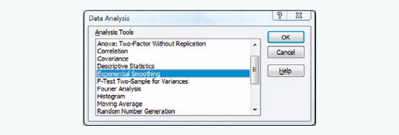
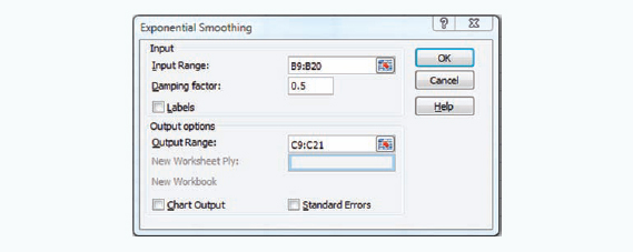
The exponential smoothing forecast can also be developed directly from Excel without "customizing" a spreadsheet and entering formulas as we did in Exhibit 12.1. From the Tools menu at the top of the spreadsheet select the "Data" option and then "Data Analysis" Option. Exhibit 12.3 shows the "Data Analysis" window and the "Exponential Smoothing" menu item, which should be selected by clicking on "OK." The resulting "Exponential Smoothing" window is shown in Exhibit 12.4. The "input range" includes the demand values in column B in Exhibit 12.1, the damping factor is α, which in this case is 0.5, and the output should be placed in column C in Exhibit 12.1. Clicking on "OK" will result in the same forecast values in column C of Exhibit 12.1 as we computed using our own exponential smoothing formula. Note that the Data Analysis group of analysis tools does not have an adjusted exponential smoothing selection; that is one reason we developed our own customized spreadsheet in Exhibit 12.1. The "Data Analysis" tools also have a moving average menu item that you can use to compute a moving average forecast.
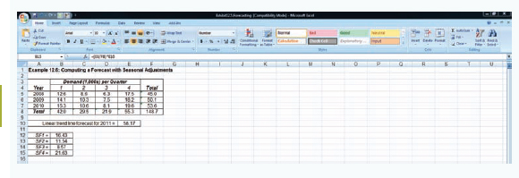
Excel can also be used to develop more customized forecast models, like seasonal forecasts. Exhibit 12.5 shows an Excel screen for the seasonal forecast model developed in Example 12.6. Notice that the computation of the seasonal forecast for the first quarter (SF1) in cell B12 is computed using the formula shown on the formula bar at the top of the screen. The forecast value for SF1 is slightly different than the value in Example 12.6 because of rounding.
OM Tools has modules for all of the forecasting methods presented in this chapter. As an example, Exhibit 12.6 shows the OM Tools spreadsheet for the exponential smoothing model (α = 0.30) in Example 12.3.
In the Institute of Business Forecasting survey we referred to previously in the section on time series methods (page 503), the second most popular forecasting technique among various industrial firms was regression. Regression is used for forecasting by establishing a mathematical relationship between two or more variables. We are interested in identifying relationships between variables and demand. If we know that something has caused demand to behave in a certain way in the past, we would like to identify that relationship so if the same thing happens again in the future, we can predict what demand will be. For example, there is a relationship between increased demand in new housing and lower interest rates. Correspondingly, a whole myriad of building products and services display increased demand if new housing starts increase.
The simplest form of regression is linear regression, which we used previously to develop a linear trend line for forecasting. Now we will show how to develop a regression model for variables related to demand other than time.
Linear regression is a mathematical technique that relates one variable, called an independent variable, to another, the dependent variable, in the form of an equation for a straight line. A linear equation has the following general form:
y = a + bx
where
y = the dependent variable
a = the intercept
b = the slope of the line
x = the independent variable
Because we want to use linear regression as a forecasting model for demand, the dependent variable, y, represents demand, and x is an independent variable that causes demand to behave in a linear manner.
To develop the linear equation, the slope, b, and the intercept, a, must first be computed using the following least squares formulas:

where
• Linear regression: a mathematical technique that relates a dependent variable to an independent variable in the form of a linear equation.
Linear regression relates demand (dependent variable) to an independent variable.
Developing a Linear Regression Forecast
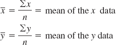
The State University athletic department wants to develop its budget for the coming year using a forecast for football attendance. Football attendance accounts for the largest portion of its revenues, and the athletic director believes attendance is directly related to the number of wins by the team. The business manager has accumulated total annual average attendance figures for the past eight years.
Wins | Attendance | Wins | Attendance |
|---|---|---|---|
4 | 36,300 | 6 | 44,000 |
6 | 40,100 | 7 | 45,600 |
6 | 41,200 | 5 | 39,000 |
8 | 53,000 | 7 | 47,500 |
Given the number of returning starters and the strength of the schedule, the athletic director believes the team will win at least seven games next year. Develop a simple regression equation for this data to forecast attendance for this level of success.
Solution
The computations necessary to compute a and b using the least squares formulas are summarized in the accompanying table. (Note that y is given in 1000s to make manual computation easier.)
x (Wins) | y (Attendance, 1000s) | xy | x2 |
|---|---|---|---|
4 | 36.3 | 145.2 | 16 |
6 | 40.1 | 240.6 | 36 |
6 | 41.2 | 247.2 | 36 |
8 | 53.0 | 424.0 | 64 |
6 | 44.0 | 264.0 | 36 |
7 | 45.6 | 319.2 | 49 |
5 | 39.0 | 195.0 | 25 |
7 | 47.5 | 332.5 | 49 |
49 | 346.9 | 2167.7 | 311 |
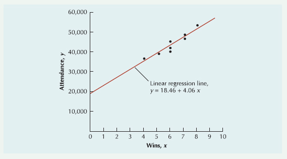
Substituting these values for a and b into the linear equation line, we have
y = 18.46 + 4.06x
Thus, for x = 7 (wins), the forecast for attendance is
The data points with the regression line are shown in the following figure. Observing the regression line relative to the data points, it would appear that the data follow a distinct upward linear trend, which would indicate that the forecast should be relatively accurate. In fact, the MAD value for this forecasting model is 1.41, which suggests an accurate forecast.
Correlation in a linear regression equation is a measure of the strength of the relationship between the independent and dependent variables. The formula for the correlation coefficient is
• Correlation: a measure of the strength of the relationship between independent and dependent variables.
The value of r varies between −1.00 and +1.00, with a value of +1.00 indicating a strong linear relationship between the variables. If r = 1.00, then an increase in the independent variable will result in a corresponding linear increase in the dependent variable. If r = −1.00, an increase in the dependent variable will result in a linear decrease in the dependent variable. A value of r near zero implies that there is little or no linear relationship between variables.
We can determine the correlation coefficient for the linear regression equation determined in Example 12.9 by substituting most of the terms calculated for the least squares formula (except for Σy2) into the formula for r:
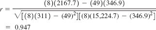
This value for the correlation coefficient is very close to 1.00, indicating a strong linear relationship between the number of wins and home attendance.
Another measure of the strength of the relationship between the variables in a linear regression equation is the coefficient of determination. It is computed by squaring the value of r. It indicates the percentage of the variation in the dependent variable that is a result of the behavior of the independent variable. For our example, r = 0.947; thus, the coefficient of determination is
This value for the coefficient of determination means that 89.7% of the amount of variation in attendance can be attributed to the number of wins by the team (with the remaining 10.3% due to other unexplained factors, such as weather, a good or poor start, or publicity). A value of 1.00 (or 100%) would indicate that attendance depends totally on wins. However, since 10.3% of the variation is a result of other factors, some amount of forecast error can be expected.
• Coefficient of determination: the percentage of the variation in the dependent variable that results from the independent variable.
The development of the simple linear regression equation and the correlation coefficient for our example was not too difficult because the amount of data was relatively small. However, manual computation of the components of simple linear regression equations can become very time-consuming and cumbersome as the amount of data increases. Excel has the capability of performing linear regression.
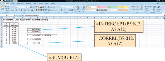
Exhibit 12.7 shows a spreadsheet set up to develop the linear regression forecast for Example 12.10 for the State University Athletic Department. Notice that Excel computes the slope directly with the formula " =SLOPE(B5:B12, A5:A12)" entered in cell E7 and shown on the formula bar at the top of the spreadsheet. The formula for the intercept in cell E6 is "=INTERCEPT(B5:B12, A5:A12)." The values for the slope and intercept are subsequently entered into cells E9 and G9 to form the linear regression equation. The correlation coefficient in cell E13 is computed using the formula "=CORREL(B5:B12, A5:A12)." Although it is not shown on the spreadsheet, the coefficient of determination (r2) could be computed using the formula "=RSQ(B5:B12, A5:A12)."
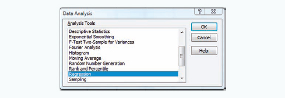
A linear regression forecast can also be developed directly with Excel using the "Data Analysis" option from the Tools menu we accessed previously to develop an exponentially smoothed forecast. Exhibit 12.8 shows the selection of "Regression" from the Data Analysis menu, and Exhibit 12.9 shows the Regression window. We first enter the cells from Exhibit 12.7 that include the y values (for attendance), B5:B12. Next enter the x value cells, A5:A12. The output range is the location on the spreadsheet where you want to put the output results. This range needs to be large (18 cells by 9 cells) and not overlap with anything else on the spreadsheet. Clicking on "OK" will result in the spreadsheet shown in Exhibit 12.10. (Note that the "Summary Output" has been slightly moved around so that all the results could be included on the screen in Exhibit 12.9).
The "Summary Output" in Exhibit 12.10 provides a large amount of statistical information, the explanation and use of which are beyond the scope of this book. The essential items that we are interested in are the intercept and slope (labeled "X Variable 1") in the "Coefficients" column at the bottom of the spreadsheet, and the "Multiple R" (or correlation coefficient) value shown under "Regression Statistics."
Another causal method of forecasting is multiple regression, a more powerful extension of linear regression. Linear regression relates demand to one other independent variable, whereas multiple regression reflects the relationship between a dependent variable and two or more independent variables. A multiple regression model has the following general form:
• Multiple regression: a relationship of demand to two or more independent variables.
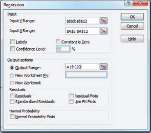
where
β0 = the intercept
β1,..., βk = parameters representing the contribution of the independent variables
x1, . . ., xk = independent variables
For example, the demand for new housing (y) in a region might be a function of several in-dependent variables, including interest rates, population, housing prices, and personal income. Development and computation of the multiple regression equation, including the compilation of data, is more complex than linear regression. The only means for forecasting using multiple regression is with a computer.
A problem often encountered in multiple regression is multicollinearity, or the amount of "overlapping" information about the dependent variable that is provided by several independent variables. This problem usually occurs when the independent variables are highly correlated, as in this example, in which wins and promotional expenditures are both positively correlated (i.e., more wins coincide with higher promotional expenditures and vice versa). (Possibly the athletic department increased promotional expenditures when it thought it would have a better team that would achieve more wins.) The topic of multicollinearity and how to cope with it is beyond the scope of this book and this brief section on multiple regression; however, most statistics textbooks discuss this topic in detail.
Forecasts of product demand are a necessity for almost all aspects of operational planning. Short-range demand forecasts determine the daily resource requirements needed for production, including labor and material, as well as for developing work schedules and shipping dates and controlling inventory levels. Long-range forecasts are needed to plan new products for development and changes in existing products and to acquire the plant, equipment, personnel, resources, and supply chain necessary for future operations.
We have presented several methods of forecasting useful for different time frames. These quantitative forecasting techniques are easy to understand, simple to use, and not especially costly unless the data requirements are substantial. They also have exhibited a good track record of performance for many companies that have used them. For these reasons, regression methods, and especially times series, are popular.
When managers and students are first introduced to forecasting methods, they are sometimes surprised and disap-pointed at the lack of exactness of the forecasts. However, they soon learn that forecasting is not easy, and exactness is not possible. Nonetheless, companies that have the skill and experience to obtain more accurate forecasts than their competitors' will gain a competitive edge.
Moving Average
Weighted Moving Average
Exponential Smoothing
Adjusted Exponential Smoothing
Trend Factor
Linear Trend Line
Least Squares
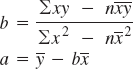
Seasonal Factor
Seasonally Adjusted Forecast
Mean Absolute Deviation
Mean Absolute Percent Deviation
Cumulative Error
Average Error (Bias)
Tracking Signal
Mean Squared Error
Linear Regression Equation
Correlation Coefficient
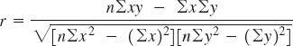
Coefficient of Determination
Coefficient of determination = r2
adjusted exponential smoothing an exponential smoothing forecast adjusted for trend.
average error the cumulative error averaged over the number of time periods.
coefficient of determination the correlation coefficient squared; it measures the portion of the variation in the dependent variable that can be attributed to the independent variable.
correlation a measure of the strength of the causal relationship between the independent and dependent variables in a linear regression equation.
cumulative error a sum of the forecast errors; also known as bias.
cycle an up-and-down movement in demand over time.
Delphi method a procedure for acquiring informed judgments and opinions from knowledgeable individuals to use as a subjective forecast.
exponential smoothing an averaging method that weights the most recent data more strongly than more distant data.
forecast error the difference between actual and forecasted demand.
linear regression a mathematical technique that relates a dependent variable to an independent variable in the form of a linear equation.
linear trend line a forecast using the linear regression equation to relate demand to time.
long-range forecast a forecast encompassing a period longer than two years into the future.
mean absolute deviation (MAD) the per-period average of the absolute difference between actual and forecasted demand.
mean absolute percent deviation (MAPD) the absolute forecast error measured as a percentage of demand.
mean squared error (MSE) the average of the squared forecast errors.
moving average average demand for a fixed sequence of periods including the most recent period.
multiple regression a mathematical relationship that relates a dependent variable to two or more independent variables.
qualitative forecast methods nonquantitative, subjective forecasts based on judgment, opinion, experience, and expert opinion.
quantitative forecast methods forecasts derived from a mathematical formula.
random variations movements in demand that are not predictable and follow no pattern.
regression forecasting methods a class of mathematical techniques that relate demand to factors that cause demand behavior.
seasonal factor a numerical value that is multiplied by the normal forecast to get a seasonally adjusted forecast.
seasonal pattern an oscillating movement in demand that occurs periodically in the short run and is repetitive.
short- to mid-range forecast a forecast encompassing the immediate future, usually days or weeks, but up to two years.
smoothing constant the weighting factor given to the most recent data in exponential smoothing forecasts.
time frame how far into the future something is forecasted.
time series methods a class of statistical methods that uses historical demand data over a period of time to predict future demand.
tracking signal a measure computed by dividing the cumulative error by MAD; used for monitoring bias in a forecast.
trend a gradual, long-term up or down movement of demand.
weighted moving average a moving average with more recent demand values adjusted with weights.
1. MOVING AVERAGE
A manufacturing company has monthly demand for one of its products as follows:
MONTH | DEMAND |
|---|---|
February | 520 |
March | 490 |
April | 550 |
May | 580 |
June | 600 |
July | 420 |
August | 510 |
September | 610 |
Develop a three-period moving average forecast and a three-period weighted moving average forecast with weights of 0.50, 0.30, and 0.20 for the most recent demand values, in that order. Calculate MAD for each forecast, and indicate which would seem to be most accurate.
SOLUTION
Step 1. Compute the three-month moving average using the formula
For May, the moving average forecast is
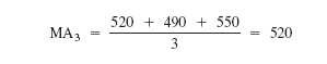
Step 2. Compute the three-month weighted moving average using the formula
WMA3 = ΣWiDi
For May, the weighted average forecast is
WMA3 = (0.50)(550) + (0.30)(490) + (0.20)(520)
= 526.00
The values for both moving average forecasts are shown in the following table:
MONTH | DEMAND | MA3 | WMA3 |
|---|---|---|---|
February | 520 | − | − |
March | 490 | − | − |
April | 550 | − | − |
May | 580 | 520.00 | 526.00 |
June | 600 | 540.00 | 553.00 |
July | 420 | 576.67 | 584.00 |
August | 510 | 533.33 | 506.00 |
September | 610 | 510.00 | 501.00 |
October | − | 513.33 | 542.00 |
Step 3. Compute the MAD value for both forecasts:
The MAD value for the three-month moving average is 80.0, and the MAD value for the three-month weighted moving average is 75.6, indicating there is not much difference in accuracy between the two forecasts, although the weighted moving average is slightly better.
2. EXPONENTIAL SMOOTHING
A computer software firm has experienced the following demand for its "Personal Finance" software package:
PERIOD | UNITS |
|---|---|
1 | 56 |
2 | 61 |
3 | 55 |
4 | 70 |
5 | 66 |
6 | 65 |
7 | 72 |
8 | 75 |
Develop an exponential smoothing forecast using α = 0.40 and an adjusted exponential smoothing forecast using α = 0.40 and β = 0.20. Compare the accuracy of the two forecasts using MAD and cumulative error.
SOLUTION
Step 1. Compute the exponential smoothing forecast with α = 0.40 using the following formula:
For period 2, the forecast (assuming F1 = 56) is
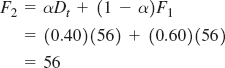
For period 3, the forecast is
The remaining forecasts are computed similarly and are shown in the accompanying table.
Step 2. Compute the adjusted exponential smoothing forecast with α = 0.40 and β = 0.20 using the formula
Starting with the forecast for period 3 (since F1 = F2, and we will assume T2 = 0),
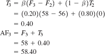
The remaining adjusted forecasts are computed similarly and are shown in the following table:
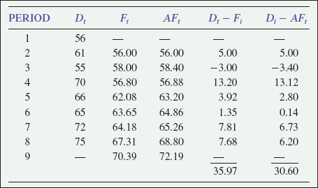
Step 3. Compute the MAD value for each forecast:
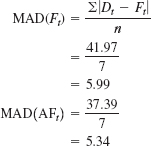
Step 4. Compute the cumulative error for each forecast:
Because both MAD and the cumulative error are less for the adjusted forecast, it would appear to be the most accurate.
3. LINEAR REGRESSION
A local building products store has accumulated sales data for 2 × 4 lumber (in board feet) and the number of building permits in its area for the past 10 quarters:
QUARTER | BUILDING PERMITS x | LUMBER SALES (1000S OF BOARD FEET)y |
|---|---|---|
1 | 8 | 12.6 |
2 | 12 | 16.3 |
3 | 7 | 9.3 |
4 | 9 | 11.5 |
5 | 15 | 18.1 |
6 | 6 | 7.6 |
7 | 5 | 6.2 |
8 | 8 | 14.2 |
9 | 101 | 15.0 |
10 | 12 | 17.8 |
Develop a linear regression model for these data and determine the strength of the linear relationship using correlation. If the model appears to be relatively strong, determine the forecast for lumber given ten building permits in the next quarter.
SOLUTION
Step 1. Compute the components of the linear regression equation, y = a + bx, using the least squares formulas
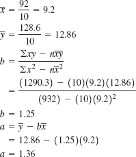
Step 2. Develop the linear regression equations:
Step 3. Compute the correlation coefficient:
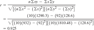
Thus, there appears to be a strong linear relationship.
Step 4. Calculate the forecast for x = 10 permits.
12-1. List some of the operations and functions in a company that are dependent on a forecast for product demand.
12-2. What is the difference between quantitative forecast methods and qualitative forecast methods?
12-3. Describe the difference between short and long-range forecasts.
12-4. Discuss the role of forecasting in supply chain management.
12-5. Why is accurate forecasting so important to companies that use a continuous replenishment inventory system?
12-6. Discuss the relationship between forecasting and quality management.
12-7. What kinds of forecasting methods are used for long-range strategic planning?
12-8. Describe the Delphi method for forecasting.
12-9. What is the difference between a trend and a cycle and a seasonal pattern?
12-10. How is the moving average method similar to exponential smoothing?
12-11. In the chapter examples for time series methods, the starting forecast was always assumed to be the same as actual demand in the first period. Suggest other ways that the starting forecast might be derived in actual use.
12-12. What effect on the exponential smoothing model will increasing the smoothing constant have?
12-13. How does adjusted exponential smoothing differ from exponential smoothing?
12-14. What determines the choice of the smoothing constant for trend in an adjusted exponential smoothing model?
12-15. How does the linear trend line forecasting model differ from a linear regression model for forecasting?
12-16. Of the time series models presented in this chapter, including the moving average and weighted moving average, exponential smoothing and adjusted exponential smoothing, and linear trend line, which one do you consider the best? Why?
12-17. What advantages does adjusted exponential smoothing have over a linear trend line for forecasted demand that exhibits a trend?
12-18. Describe how a forecast is monitored to detect bias.
12-19. Explain the relationship between the use of a tracking signal and statistical control limits for forecast control.
12-20. Selecting from MAD, MAPD, MSE, E, and, Ē which measure of forecast accuracy do you consider superior? Why?
12-21. What is the difference between linear and multiple regression?
12-22. Define the different components (y, x, a, and b) of a linear regression equation.
12-23. A company that produces video equipment, including video cameras and televisions, is attempting to forecast what new products and product innovations might be technologically feasible and that customers might demand 10 years into the future. Speculate on what type of qualitative methods it might use to develop this type of forecast.
12-1. The Hartley-Davis motorcycle dealer in the Minneapolis– St. Paul area wants to be able to forecast accurately the demand for the Roadhog Super motorcycle during the next month. From sales records, the dealer has accumulated the data in the following table for the past year.
Month | Motorcycle Sales |
|---|---|
January | 9 |
February | 7 |
March | 10 |
April | 8 |
May | 7 |
June | 12 |
July | 10 |
August | 11 |
September | 12 |
October | 10 |
November | 14 |
December | 16 |
Compute a three-month moving average forecast of demand for April through January (of the next year).
Compute a five-month moving average forecast for June through January.
Compare the two forecasts computed in parts (a) and (b) using MAD. Which one should the dealer use for January of the next year?
12-2. The manager of the I-85 Carpet outlet needs to be able to forecast accurately the demand for Soft Shag carpet (its biggest seller). If the manager does not order enough carpet from the carpet mill, customers will buy their carpets from one of the outlets many competitors. The manager has collected the following demand data for the past eight months.
Month | Demand for Soft Shag Carpet (1000 yd) |
|---|---|
1 | 5 |
2 | 10 |
3 | 6 |
4 | 8 |
5 | 14 |
6 | 10 |
7 | 9 |
8 | 12 |
Compute a three-month moving average forecast for months 4 through 9.
Compute a weighted three-month moving average forecast for months 4 through 9. Assign weights of 0.55, 0.33, and 0.12 to the months in sequence, starting with the most recent month.
Compare the two forecasts using MAD. Which forecast appears to be more accurate?
12-3. The LawnPlus Fertilizer Company distributes fertilizer to various lawn and garden shops. The company must base its quarterly production schedule on a forecast of how many tons of fertilizer will be demanded from it. The company has gathered the following data for the past three years from its sales records.
Year | Quarter | Demand for Fertilizer (ton) |
|---|---|---|
1 | 1 | 105 |
2 | 150 | |
3 | 93 | |
4 | 121 | |
2 | 5 | 140 |
6 | 170 | |
7 | 105 | |
8 | 150 | |
3 | 9 | 150 |
10 | 170 | |
11 | 110 | |
12 | 130 |
Compute a three-quarter moving average forecast for quarters 4 through 13 and compute the forecast error for each quarter.
Compute a five-quarter moving average forecast for quarters 6 through 13 and compute the forecast error for each quarter.
Compute a weighted three-quarter moving average forecast using weights of 0.50, 0.33, and 0.17 for the most recent, next recent, and most distant data, respectively, and compute the forecast error for each quarter.
Compare the forecasts developed in parts (a), (b), and (c) using cumulative error. Which forecast appears to be most accurate? Do any exhibit any bias?
12-4. Graph the demand data in Problem 12-3. Can you identify any trends, cycles, and/or seasonal patterns?
12-5. The chairperson of the department of management at Tech wants to forecast the number of students who will enroll in operations management next semester in order to determine how many sections to schedule. The chair has accumulated the following enrollment data for the past eight semesters:
Semester | Students Enrolled in OM |
|---|---|
1 | 270 |
2 | 310 |
3 | 250 |
4 | 290 |
5 | 370 |
6 | 410 |
7 | 400 |
8 | 450 |
Compute a three-semester moving average forecast for semesters 4 through 9.
Compute the exponentially smoothed forecast (α = 0.20) for the enrollment data.
Compare the two forecasts using MAD and indicate the most accurate.
12-6. The manager of the Excom Service Station wants to forecast the demand for unleaded gasoline next month so that the proper number of gallons can be ordered from the distributor. The owner has accumulated the following data on demand for unleaded gasoline from sales during the past 10 months:
Month | Gasoline Demanded (gal) |
|---|---|
October | 800 |
November | 725 |
December | 630 |
January | 500 |
February | 645 |
March | 690 |
April | 730 |
May | 810 |
June | 1200 |
July | 980 |
Compute an exponentially smoothed forecast using an α value of 0.30.
Compute an adjusted exponentially smoothed forecast (α = 0.30 and β = 0.20).
Compare the two forecasts using MAPD and indicate which seems to be the most accurate.
12-7. The Intrepid mutual fund of growth stocks has had the following average monthly price for the past 10 months.
Month | Fund Price |
|---|---|
1 | 62.7 |
2 | 63.9 |
3 | 68.0 |
4 | 66.4 |
5 | 67.2 |
6 | 65.8 |
7 | 68.2 |
8 | 69.3 |
9 | 67.2 |
10 | 70.1 |
Compute the exponentially smoothed forecast with α = 0.40, the adjusted exponentially smoothed forecast with α = 0.40 and β = 0.30, and the linear trend line forecast. Compare the accuracy of the three forecasts using cumulative error and MAD, and indicate which forecast appears to be most accurate.
12-8. The Oceanside Hotel is adjacent to City Coliseum, a 24,000-seat arena that is home to the city's professional basketball and ice hockey teams and that hosts a variety of concerts, trade shows, and conventions throughout the year. The hotel has experienced the following occupancy rates for the nine years since the coliseum opened:
Year | Occupancy Rate |
|---|---|
1 | 75% |
2 | 70 |
3 | 72 |
4 | 77 |
5 | 83 |
6 | 81 |
7 | 86 |
8 | 91 |
9 | 87 |
Compute an exponential smoothing forecast with α = 0.20, an adjusted exponential smoothing forecast with α = 0.20 and β = 0.20, and a linear trend line forecast. Compare the three forecasts using MAD and average error (Ē), and indicate which forecast seems to be most accurate.
12-9. Mary Hernandez has invested in a stock mutual fund and she is considering liquidating and investing in a bond fund. She would like to forecast the price of the stock fund for the next month before making a decision. She has collected the following data on the average price of the fund during the past 20 months.
Month | Fund Price | Month | Fund Price |
|---|---|---|---|
1 | 63 1/4 | 11 | 68 1/8 |
2 | 60 1/8 | 12 | 63 1/4 |
3 | 61 3/4 | 13 | 64 3/8 |
4 | 64 1/4 | 14 | 68 5/8 |
5 | 59 3/8 | 15 | 70 1/8 |
6 | 57 7/8 | 16 | 72 3/4 |
7 | 62 1/4 | 17 | 74 1/8 |
8 | 65 1/8 | 18 | 71 3/4 |
9 | 68 1/4 | 19 | 75 1/2 |
10 | 65 1/2 | 20 | 76 3/4 |
Using a three-month moving average, forecast the fund price for month 21.
Using a three-month weighted average with the most recent month weighted 0.60, the next most recent month weighted 0.30, and the third month weighted 0.10, forecast the fund price for month 21.
Compute an exponentially smoothed forecast using α = 0.40 and forecast the fund price for month 21.
Compare the forecasts in (a), (b), and (c) using MAD and indicate the most accurate.
12-10. Globetron manufactures components for use in small electronic products such as computers, CD players, and radios at plants in Belgium, Germany, and France. The parts are transported by truck to Hamburg, where they are shipped overseas to customers in Mexico, South America, the United States, and the Pacific Rim. The company has to reserve space on ships, months and sometimes years in advance, and as such needs an accurate forecasting model. Following are the number of cubic feet of container space the company has used in each of the past 18 months.
Month | Space (1000s ft3) | Month | Space (1000s ft3) |
|---|---|---|---|
1 | 10.6 | 10 | 19.2 |
2 | 12.7 | 11 | 16.3 |
3 | 9.8 | 12 | 14.7 |
4 | 11.3 | 13 | 18.2 |
5 | 13.6 | 14 | 19.6 |
6 | 14.4 | 15 | 21.4 |
7 | 12.2 | 16 | 22.8 |
8 | 16.7 | 17 | 20.6 |
9 | 18.1 | 18 | 18.7 |
Develop a forecasting model that you believe would provide the company with relatively accurate forecasts for the next year and indicate the forecasted shipping space required for the next three months.
12-11. The Bee Line Café is well known for its popular homemade ice cream, which it makes in a small plant in back of the cafe. People drive long distances to buy the ice cream. The two ladies who own the café want to develop a forecasting model so they can plan their ice cream production operation and determine the number of employees they need to sell ice cream in the café. They have accumulated the following sales records for their ice cream for the past 12 quarters:
Year/Quarter | Ice Cream Sales (gal) |
|---|---|
2008:1 | 350 |
2 | 510 |
3 | 750 |
4 | 420 |
2009:5 | 370 |
6 | 480 |
7 | 860 |
8 | 500 |
2010:9 | 450 |
10 | 550 |
11 | 820 |
12 | 570 |
Develop an adjusted exponential smoothing model with α = 0.50 and β = 0.50 to forecast demand, and assess its accuracy using cumulative error (E) and average error (Ē). Does there appear to be any bias in the forecast?
12-12. For the demand data in Problem 12-11, develop a seasonally adjusted forecast for 2011. (Use a linear trend line model to develop a forecast estimate for 2005.) Which forecast model do you perceive to be the most accurate, the adjusted exponential smoothing model from Problem 12- 11 or the seasonally adjusted forecast?
12-13. Develop a seasonally adjusted forecast for the demand data for fertilizer in Problem 12-3. Use a linear trend line model to compute a forecast estimate for demand in year 4.
12-14. Backstreet's Pizza delivery service has randomly selected eight weekdays during the past month and recorded orders for pizza at four different time periods per day, as follows:
Time Period | Days | |||||||
|---|---|---|---|---|---|---|---|---|
1 | 2 | 3 | 4 | 5 | 6 | 7 | 8 | |
10:00 A.M.–3:00 P.M. | 62 | 49 | 53 | 35 | 43 | 48 | 56 | 43 |
3:00 P.M.–7:00 P.M. | 73 | 55 | 81 | 77 | 60 | 66 | 85 | 70 |
7:00 P.M.–11:00 P.M. | 42 | 38 | 45 | 50 | 29 | 37 | 35 | 44 |
11:00 P.M.–2:00 P.M. | 35 | 40 | 36 | 39 | 26 | 25 | 36 | 31 |
Develop a seasonally adjusted forecasting model for daily pizza demand and forecast demand for each of the time periods for a single upcoming day.
12-15. The Willow River Mining Company mines and ships coal. It has experienced the following demand for coal during the past eight years:
Year | Coat Sales (tons) |
|---|---|
1 | 4260 |
2 | 4510 |
3 | 4050 |
4 | 3720 |
5 | 3900 |
6 | 3470 |
7 | 2890 |
8 | 3100 |
Develop an adjusted exponential smoothing model (α = 0.30, β = 0.20) and a linear trend line model, and compare the forecast accuracy of the two using MAD. Indicate which forecast seems to be most accurate.
12-16. The Great Northwest Outdoor Company is a catalogue sales operation that specializes in outdoor recreational clothing. Demand for its items is very seasonal, peaking during the holiday season and during the spring. It has accumulated the following data for order per "season" (quarter) during the past five years:
Orders (1000s) | |||||
|---|---|---|---|---|---|
Quarter | 2006 | 2007 | 2008 | 2009 | 2010 |
January-March | 18.6 | 18.1 | 22.4 | 23.2 | 24.5 |
April-June | 23.5 | 24.7 | 28.8 | 27.6 | 31.0 |
July-September | 20.4 | 19.5 | 21.0 | 24.4 | 23.7 |
October-December | 41.9 | 46 3 | 45.5 | 47.1 | 52.8 |
Develop a seasonally adjusted forecast model for these order data. Forecast demand for each quarter for 2011 (using a linear trend line forecast estimate for orders in 2011).
Develop a separate linear trend line forecast for each of the four seasons and forecast each season for 2011.
Which of the two approaches used in parts (a) and (b) appear to be the most accurate? Use MAD to verify your selection.
12-17. Townside Food Vending operates vending machines in office buildings, the airport, bus stations, colleges, and other businesses and agencies around town and operates vending trucks for building and construction sites. The company believes its sandwich sales follow a seasonal pattern. It has accumulated the following data for sandwich sales per season during the past four years.
Sandwich Sales (1000s) | ||||
|---|---|---|---|---|
Season | 2007 | 2008 | 2009 | 2010 |
Fall | 42.7 | 44.3 | 45.7 | 40.6 |
Winter | 36.9 | 42.7 | 34.8 | 41.5 |
Spring | 51.3 | 55.6 | 49.3 | 47.3 |
Summer | 62.9 | 64.8 | 71.2 | 74.5 |
Develop a seasonally adjusted forecast model for these sandwich sales data. Forecast demand for each season for 2011 using a linear trend line estimate for sales in 2011. Do the data appear to have a seasonal pattern?
12-18. The town aquatic center has an indoor pool that has lanes for lap swimming and an open area for recreational swimming and water exercises. When local schools are in session from mid-August to late May, during weekdays the pool operates from 7:00 A.M. to 9:00 P.M. The center requires a lifeguard to pool user ratio of 30:1. The center director has to submit a new yearly budget to the town and wants to develop a forecast of hourly pool attendance in order to determine the number of lifeguards she'll have to hire in the coming year. The director believes pool attendance follows a seasonal pattern during the day and she has accumulated the following data for average daily attendance for each hour of the day that the pool is open to the public for the past six years.
Year | ||||||
|---|---|---|---|---|---|---|
Time | 1 | 2 | 3 | 4 | 5 | 6 |
7:00 A.M. | 56 | 64 | 66 | 60 | 72 | 65 |
8:00 | 31 | 41 | 37 | 44 | 52 | 46 |
9:00 | 15 | 22 | 24 | 30 | 19 | 26 |
10:00 | 34 | 35 | 38 | 31 | 28 | 33 |
11:00 | 45 | 52 | 55 | 49 | 57 | 50 |
Noon | 63 | 71 | 57 | 65 | 75 | 70 |
1:00 P.M. | 35 | 30 | 41 | 42 | 33 | 45 |
2:00 | 24 | 28 | 32 | 30 | 35 | 33 |
3:00 | 27 | 19 | 24 | 23 | 25 | 27 |
6:00 | 31 | 47 | 36 | 45 | 40 | 46 |
7:00 | 25 | 35 | 41 | 43 | 39 | 45 |
8:00 | 14 | 20 | 18 | 17 | 23 | 27 |
9:00 | 10 | 8 | 16 | 14 | 15 | 18 |
Develop a seasonally adjusted forecast for these data for hourly pool attendance. Forecast average pool attendance for each hour for year 7 by using a linear trend line estimate for pool attendance in year 7. Do the data appear to have a seasonal pattern?
12-19. Develop an adjusted exponential smoothing forecast (α = .30, β = .20) for the annual pool attendance data in Problem 12-18. Does this forecast appear to be more or less accurate than the forecast based on the linear trend line model to forecast hourly pool attendance in Problem S-18?
12-20. During the past five months the emergency room at the new County Hospital has observed the number of patients during two parts of every other week—the weekend (Friday through Sunday) and weekdays (Monday through Thursday). They typically experience greater patient traffic on weekends than during the week:
Number of Patients | ||
|---|---|---|
Week | Weekend | Weekdays |
1 | 105 | 73 |
2 | 119 | 85 |
3 | 122 | 89 |
4 | 128 | 83 |
5 | 117 | 96 |
6 | 136 | 78 |
7 | 141 | 91 |
8 | 126 | 100 |
9 | 143 | 83 |
10 | 140 | 101 |
Develop a seasonally adjusted forecasting model for number of patients during each part of the week for week 11.
12-21. Temco Industries has developed a forecasting model that was used to forecast during a ten-month period. The forecasts and actual demand are shown as follows:
Month | Actual Demand | Forecast Demand |
|---|---|---|
1 | 160 | 170 |
2 | 150 | 165 |
3 | 175 | 157 |
4 | 200 | 166 |
5 | 190 | 183 |
6 | 220 | 186 |
7 | 205 | 203 |
8 | 210 | 204 |
9 | 200 | 207 |
10 | 220 | 203 |
Measure the accuracy of the forecast using MAD, MAPD, and cumulative error. Does the forecast method appear to be accurate?
12-22. Monitor the forecast in Problem 12-21 for bias using a tracking signal and a control chart with ±3 MAD. Does there appear to be any bias in the forecast?
12-23. Develop a statistical control chart for the forecast error in Problem 12-11 using 63σ control limits, and indicate if the forecast seems to be biased.
12-24. Monitor the adjusted exponential smoothing forecast in Problem 12-15 for bias using a tracking signal and a control chart with ±3 MAD.
12-25. RAP Computers assembles computers from generic parts it purchases at discount and sells the units via phone orders it receives from customers responding to their ads in trade journals. The business has developed an exponential smoothing forecast model to forecast future computer demand. Actual demand for their computers for the past eight months is as follows:
Month | Demand | Forecast |
|---|---|---|
March | 120 | − |
April | 110 | 120.0 |
May | 150 | 116.0 |
June | 130 | 129.6 |
July | 160 | 129.7 |
August | 165 | 141.8 |
September | 140 | 151.1 |
October | 155 | 146.7 |
November | − | 150.0 |
Using the measure of forecast accuracy of your choice, ascertain if the forecast appears to be accurate.
Determine if a three-month moving average would provide a better forecast.
Use a tracking signal to monitor the forecast in part (a) for bias.
12-26. Develop an exponential smoothing forecast with α = 0.20 for the demand data in Problem 12-1. Compare this forecast with the three-month moving average computed in 12-1(a) using MAD and indicate which forecast seems to be most accurate.
12-27. The Fieldale Dairy produces cheese, which it sells to supermarkets and food processing companies. Because of concerns about cholesterol and fat in cheese, the company has seen demand for its products decline during the past decade. It is now considering introducing some alternative low-fat dairy products and wants to determine how much available plant capacity it will have next year. The company has developed an exponential smoothing forecast with α = 0.40 to forecast cheese. The actual demand and the forecasts from its model are shown as follows:
Demand | ||
|---|---|---|
Year | (1000s lb) | Forecast |
1 | 16.8 | − |
2 | 14.1 | 16.8 |
3 | 15.3 | 15.7 |
4 | 12.7 | 15.5 |
5 | 11.9 | 14.4 |
6 | 12.3 | 13.4 |
7 | 11.5 | 12.9 |
8 | 10.8 | 12.4 |
Assess the accuracy of the forecast model using MAD and cumulative error, and determine if the forecast error reflects bias using a tracking signal and ±3 MAD control limits. If the exponential smoothing forecast model is biased, determine if a linear trend model would provide a more accurate forecast.
12-28. The manager of the Commander Hotel near City Stadium believes that how well the local Blue Sox professional baseball team is playing has an impact on the occupancy rate at the hotel during the summer months. Following are the number of victories for the Blue Sox (in a 162-game schedule) for the past eight years and the hotel occupancy rates:
Year | Number of Blue Sox Wins | Occupancy Rate |
|---|---|---|
1 | 70 | 81% |
2 | 65 | 74 |
3 | 81 | 83 |
4 | 88 | 84 |
5 | 80 | 85 |
6 | 92 | 91 |
7 | 83 | 88 |
8 | 64 | 80 |
Develop a linear regression model for these data, and forecast the occupancy rate for next year if the Blue Sox win 85 games. Does there appear to be a strong relationship between wins and occupancy rate?
12-29. The I-85 Carpet Outlet wants to develop a means to forecast its carpet sales. The store manager believes that the store's sales are directly related to the number of new housing starts in town. The manager has gathered data from county records of monthly house construction permits and from store records on monthly sales. These data are as follows:
Monthly Carpet Sales (1000s yd) | Monthly Construction Permits |
|---|---|
5 | 17 |
12 | 30 |
6 | 12 |
5 | 14 |
8 | 18 |
4 | 10 |
14 | 38 |
9 | 20 |
9 | 16 |
16 | 31 |
Develop a linear regression model for this data and forecast carpet sales if 25 construction permits for new homes are filed.
Determine the strength of the causal relationship between monthly sales and new home construction using correlation.
12-30. The manager of Sarah's Ice Cream store needs an accurate forecast of the demand for ice cream. The store orders ice cream from a distributor a week ahead, and if too little is ordered the store loses business. If it orders too much, it must be thrown away. The manager believes that a major determinant of ice cream sales is temperature; that is, the hotter it is, the more ice cream people buy. Using an almanac, the manager has determined the average daytime temperature for 10 weeks selected at random and then, from store records, has determined the ice cream consumption for the same 10 weeks. The data are summarized as follows:
Week | Temperature | (Gallons Sold) |
|---|---|---|
1 | 75 | 95 |
2 | 67 | 90 |
3 | 83 | 125 |
4 | 89 | 150 |
5 | 77 | 85 |
6 | 80 | 115 |
7 | 84 | 110 |
8 | 92 | 145 |
9 | 89 | 130 |
10 | 65 | 100 |
Develop a linear regression model for this data and forecast the ice cream consumption if the average weekly daytime temperature is expected to be 80.
Determine the strength of the linear relationship between temperature and ice cream consumption using correlation.
12-31. Compute the coefficient of determination for the data in Problem 12-30 and explain its meaning.
12-32. The registrar at State University believes that decreases in the number of freshman applications that have been experienced are directly related to tuition increases. They have collected the following enrollment and tuition data for the past decade:
Year | Freshman Applications | Annual Tuition ($) |
|---|---|---|
1 | 6010 | 3600 |
2 | 5560 | 3600 |
3 | 6100 | 4000 |
4 | 5330 | 4400 |
5 | 4980 | 4500 |
6 | 5870 | 5700 |
7 | 5120 | 6000 |
8 | 4750 | 6000 |
9 | 4615 | 7500 |
10 | 4100 | 8000 |
Develop a linear regression model for these data and forecast the number of applications for State University if tuition increases to $10,000 per year and if tuition is lowered to $7000 per year.
Determine the strength of the linear relationship between freshman applications and tuition using correlation.
Describe the various planning decisions for State University that would be affected by the forecast for freshman applications.
12-33. Employees at Hubbell Engine Parts Company produce parts using precision machine tools according to exact design specifications. The employees are paid partially according to a piece rate system wherein if they work faster and produce more parts, they are eligible for monthly bonuses. Management suspects that this method of pay may contribute to a high number of defective parts. A specific part requires a normal, standard time of 23 minutes to produce. The quality control manager has checked the actual average times to produce this part for 10 different employees during 20 days selected at random during the past month, and determined the corresponding percentage of defective parts, as follows.
Average Time (min) | % Defective | Average Time (min) | % Defective |
|---|---|---|---|
21.6 | 4.1 | 20.8 | 3.1 |
22.5 | 4.6 | 18.9 | 6.1 |
23.1 | 1.2 | 21.4 | 3.8 |
24.6 | 1.5 | 23.7 | 1.9 |
22.8 | 2.6 | 23.8 | 1.7 |
23.7 | 1.9 | 24.9 | 0.8 |
20.9 | 3.7 | 19.8 | 4.3 |
19.7 | 5.3 | 19.7 | 5.1 |
24.5 | 1.8 | 21.2 | 3.9 |
26.7 | 2.3 | 20.8 | 1.7 |
Develop a linear regression model relating average production time to percentage defects to determine if a relationship exists, and the percentage of defective items that would be expected with the normal production time of 23 minutes.
12-34. Apperson and Fitz is a chain of clothing stores that caters to high school and college students. It publishes a quarterly catalogue and operates a Web site that features provocatively attired males and females. The Web site is very expensive to maintain, and company executives are not sure if the number of hits at the site relate to sales; that is, people may be looking at the site for the pictures rather than as potential customers. The Web master has accumulated the following data for hits per month and orders placed at the Web site for the past 20 months.
Hits (1000s) | Orders (1000s) | Hits (1000s) | Orders (1000s) |
|---|---|---|---|
34.2 | 8.2 | 46.7 | 9.1 |
28.5 | 5.7 | 43.5 | 7.2 |
36.7 | 9.1 | 52.6 | 10.7 |
42.3 | 7.5 | 61.8 | 9.3 |
25.8 | 6.3 | 37.3 | 3.1 |
52.3 | 10.4 | 28.9 | 4.4 |
35.2 | 7.5 | 26.4 | 5.2 |
27.9 | 6.2 | 39.4 | 6.8 |
31.4 | 4.8 | 44.7 | 8.4 |
29.4 | 5.3 | 46.3 | 7.9 |
Develop a linear regression model for these data and indicate if there appears to be a strong relationship between Web site hits and orders. What would be the forecast for orders with 60,000 hits per month?
12-35. Develop a linear trend line model for the freshman applications data at State University in Problem 12-32.
Does this forecast appear to be more or less accurate than the linear regression forecast developed in Problem 12-32? Justify your answer.
Compute the correlation coefficient for the linear trend line forecast and explain its meaning.
12-36. Explain what the numerical value of the slope of the linear regression equation in Problem 12-30 means.
12-37. ITown is a large computer discount store that sells computers and ancillary equipment and software in the town where State University is located. It has collected historical data on computer sales and printer sales for the past 10 years as follows:
Year | Personal Computer Sales | Printers Sold |
|---|---|---|
1 | 1045 | 381 |
2 | 1610 | 579 |
3 | 860 | 312 |
4 | 1211 | 501 |
5 | 975 | 296 |
6 | 1117 | 415 |
7 | 1066 | 535 |
8 | 1310 | 592 |
9 | 1517 | 607 |
10 | 1246 | 473 |
Develop a linear trend line forecast to forecast printer demand in year 11.
Develop a linear regression model relating printer sales to computer sales to forecast printer demand in year 11 if 1500 computers are sold.
Compare the forecasts developed in parts (a) and (b) and indicate which one appears to be the best.
12-38. Develop an exponential smoothing model with α = 0.30 for the data in Problem 12-37 to forecast printer demand in year 11, and compare its accuracy to the linear regression forecast developed in Problem 12-37(a).
12-39. Arrow Air is a regional East Coast airline. It has collected data for the percentage of available seats occupied on its flights for four quarters—(1) January–March, (2) April–June, (3) July–September, and (4) October–December—for the past five years. The company also has collected data for the average percentage fare discount for each of these quarters as follows:
Year | Quarter | % Seat Occupancy | % Average Fare Discount |
|---|---|---|---|
1 | 1 | 63 | 21 |
2 | 75 | 34 | |
3 | 76 | 18 | |
4 | 58 | 26 | |
2 | 1 | 59 | 18 |
2 | 62 | 40 | |
3 | 81 | 25 | |
4 | 76 | 30 | |
3 | 1 | 65 | 23 |
2 | 70 | 28 | |
3 | 78 | 30 | |
4 | 69 | 35 | |
4 | 1 | 59 | 20 |
2 | 61 | 35 | |
3 | 83 | 26 | |
4 | 71 | 30 | |
5 | 1 | 60 | 25 |
2 | 66 | 37 | |
3 | 86 | 25 | |
4 | 74 | 30 |
Develop a seasonally adjusted forecast model for seat occupancy. Forecast seat occupancy for year 6 (using a linear trend line forecast estimate for seat occupancy in year 6).
Develop linear regression models relating seat occupancy to discount fares to forecast seat occupancy for each quarter in year 6. Assume a fare discount of 20% for quarter 1, 36% for quarter 2, 25% for quarter 3, and 30% for quarter 4.
Compare the forecasts developed in parts (a) and (b) and indicate which one appears to be the best.
12-40. Develop an adjusted exponential smoothing forecast model (α = 0.40 and β = 0.40) for the data in Problem 12-39 to forecast seat occupancy, and compare its accuracy with the seasonally adjusted model developed in Problem 12.39(a).
12-41. The consumer loan department at National Bank wants to develop a forecasting model to help determine its potential loan application volume for the coming year. Since adjustable-rate home mortgages are based on government long-term Treasury note rates, the bank has collected the following data for three- to five-year Treasury note interest rates for the past 24 years:
Year | Rate | Year | Rate | Year | Rate |
|---|---|---|---|---|---|
1 | 5.77 | 9 | 9.71 | 17 | 7.68 |
2 | 5.85 | 10 | 11.55 | 18 | 8.26 |
3 | 6.92 | 11 | 14.44 | 19 | 8.55 |
4 | 7.82 | 12 | 12.92 | 20 | 8.26 |
5 | 7.49 | 13 | 10.45 | 21 | 6.80 |
6 | 6.67 | 14 | 11.89 | 22 | 6.12 |
7 | 6.69 | 15 | 9.64 | 23 | 5.48 |
8 | 8.29 | 16 | 7.06 | 24 | 6.09 |
Develop an appropriate forecast model for the bank to use to forecast Treasury note rates in the future, and indicate how accurate it appears to be compared to historical data.
12-42. The Vantage Fund is a balanced mutual fund that includes a mix of stocks and bonds. Following are the year-end share prices of the fund and Dow Jones Industrial Average for a 20-year period.
Year | Share Price | DJIA | Year | Share Price | DJIA |
|---|---|---|---|---|---|
1 | 14.75 | 1046 | 11 | 19.08 | 3301 |
2 | 15.06 | 1258 | 12 | 20.40 | 3754 |
3 | 14.98 | 1211 | 13 | 19.39 | 3834 |
4 | 15.73 | 1546 | 14 | 24.43 | 5117 |
5 | 16.11 | 1895 | 15 | 26.46 | 6448 |
6 | 16.07 | 1938 | 16 | 29.45 | 7908 |
7 | 16.78 | 2168 | 17 | 29.35 | 9181 |
8 | 17.69 | 2753 | 18 | 27.96 | 11497 |
9 | 16.90 | 2633 | 19 | 28.21 | 10786 |
10 | 17.81 | 3168 | 20 | 27.26 | 10150 |
Develop a linear regression model for these data and forecast the fund share price for a DJIA of 12,000. Does there appear to be a strong relationship between the fund's share price and the DJIA?
12-43. The admission data for freshmen at Tech during the past 10 years are as follows:
Year | Applicants | Offers | % Offers | Acceptances | % Acceptances |
|---|---|---|---|---|---|
1 | 13,876 | 11,200 | 80.7 | 4112 | 36.7 |
2 | 14,993 | 11,622 | 77.8 | 4354 | 37.3 |
3 | 14,842 | 11,579 | 78.0 | 4755 | 41.1 |
4 | 16,285 | 13,207 | 81.1 | 5068 | 38.0 |
5 | 16,922 | 11,382 | 73.2 | 4532 | 39.8 |
6 | 16,109 | 11,937 | 74.1 | 4655 | 39.0 |
7 | 15,883 | 11,616 | 73.1 | 4659 | 40.1 |
8 | 18,407 | 11,539 | 62.7 | 4620 | 40.0 |
9 | 18,838 | 13,138 | 69.7 | 5054 | 38.5 |
10 | 17,756 | 11,952 | 67.3 | 4822 | 40.3 |
Tech's admission objective is a class of 5000 entering freshmen, and it wants to forecast the percentage of offers it will likely have to make in order to achieve this objective.
Develop a linear trend line to forecast next year's applicants and percentage acceptances and use these results to estimate the percentage offers that Tech should expect to make.
Develop a linear trend line to forecast the percentage offers that Tech should expect to make and compare this result with the result in part (a). Which forecast do you think is more accurate?
Assume Tech receives 18,300 applicants in year 11. How many offers do you think it should make to get 5000 acceptances?
12-44. The Port of Charleston is considering an expansion of their container terminal. The port has experienced the following container throughput during the past 12 years, expressed as TEUs (i.e., 20 feet equivalent units, a standard unit of measure for containers).
Year | TEUs (1,000s) |
|---|---|
1 | 526.1 |
2 | 549.4 |
3 | 606.0 |
4 | 627.0 |
5 | 695.7 |
6 | 734.9 |
7 | 761.1 |
8 | 845.4 |
9 | 1,021.1 |
10 | 1,137.1 |
11 | 1,173.6 |
12 | 1,233.4 |
Develop a linear trend line forecast for these data and forecast the number of TEUs for the next year.
How strong is the linear relationship for these data?
12-45. The County Arsenal Travel Soccer Club has boys and girls travel soccer teams at all age levels up to 18 years old. The club has been successful and grown in popularity over the years; however, an obstacle to its continued growth is a shortage of practice and game soccer fields in the area. The club has tried to make a case to the County Board of Supervisors for more soccer fields to accommodate the increasing number of kids who want to play on a club travel team. The number of kids who have played soccer on a club team, and the county's population, for the last 10 years is as follows.
Year | Club Soccer Players | Town Population |
|---|---|---|
1 | 246 | 38,060 |
2 | 235 | 38,021 |
3 | 259 | 38,110 |
4 | 261 | 38,125 |
5 | 276 | 38,240 |
6 | 290 | 38,231 |
7 | 327 | 38,306 |
8 | 318 | 38,477 |
9 | 335 | 38,506 |
10 | 331 | 38,583 |
11 | 339 | 38,609 |
12 | 351 | 38,745 |
13 | 366 | 39,003 |
14 | 401 | 39,062 |
15 | 427 | 39,114 |
The soccer club wants to develop a forecasting model to demonstrate to the Board of Supervisors its expected growth in the future.
Develop a linear trend line forecast to predict the number of soccer players the club can expect next year.
The county planning department has told the soccer club that the county expects to grow to a population of 39,300 by next year and to 40,000 in five years. Develop a linear regression model using the county's population as a predictor of the number of club soccer players and compare this forecasting model to the one developed in part (a). Which forecasting model should the club use to support its request for new fields?
12-46. The Dean of the College of Business at State University has initiated a fund raising campaign. One of the selling points she plans to use with potential donors is that increasing the college's private endowment will improve its ranking among business schools as published in various news magazines. She would like to demonstrate that there is a relationship between funding and the rankings. She has collected the following data showing the private endowments ($ millions), and annual budgets ($ millions) from state and private sources, for eight of State's peer institutions plus State, and the ranking of each school.
Private Endowment | Annual Budget | Ranking |
|---|---|---|
2.5 | 8.1 | 87 |
52.0 | 26.0 | 20 |
12.7 | 7.5 | 122 |
63.0 | 33.0 | 32 |
46.0 | 12.0 | 54 |
27.1 | 16.1 | 76 |
23.3 | 17.0 | 103 |
46.4 | 14.9 | 40 |
48.9 | 21.8 | 98 |
Use Excel to develop a linear regression model for the amount of the private endowment and the ranking, and forecast a ranking for a private endowment of $70 million. Does there appear to be a strong relationship between the endowment and ranking?
Using Excel, develop a multiple regression equation for all of these data including private endowment and annual budget, and forecast a ranking for a private endowment of $70 million and an annual budget of $40 million. How does this forecast compare to the forecast in part (a)?
12-47. Some members of management of the Fairface Cosmetics Firm believe that demand for its products is related to the promotional activities of local department stores where its cosmetics are sold. However, others in management believe that other factors, such as local demographics, are stronger determinants of demand behavior. The following data for local annual promotional expenditures for all Fairface products and local annual unit sales for Fairface lip gloss have been collected from 20 stores selected at random from different localities:
Store | Annual Unit Sales ($1000s) | Annual Promotional Expenditures ($1000s) |
|---|---|---|
1 | 5.3 | 12.6 |
2 | 4.2 | 15.5 |
3 | 3.1 | 10.8 |
4 | 2.7 | 8.7 |
5 | 5.9 | 20.3 |
6 | 5.6 | 21.9 |
7 | 10.3 | 25.6 |
8 | 4.1 | 14.3 |
9 | 9.9 | 15.1 |
10 | 5.7 | 18.7 |
11 | 3.5 | 9.6 |
12 | 3.2 | 12.7 |
13 | 8.1 | 16.3 |
14 | 3.6 | 8.1 |
15 | 5.3 | 7.5 |
16 | 5.8 | 12.4 |
17 | 8.1 | 17.3 |
18 | 6.1 | 11.2 |
19 | 3.1 | 18.5 |
20 | 9.5 | 16.7 |
Based on these data, does it appear that the strength of the relationship between lip gloss sales and promotional expenditures is sufficient to warrant using a linear regression forecasting model? Explain your response.
12-48. The Pro Apparel company manufactures baseball-style caps with various team logos. The caps come in an assortment of designs and colors. The company has had monthly sales for the past 24 months as follows:
Month | Demand (1000s) | Month | Demand (1000s) |
|---|---|---|---|
1 | 8.2 | 13 | 10.3 |
2 | 7.5 | 14 | 10.5 |
3 | 8.1 | 15 | 11.7 |
4 | 9.3 | 16 | 9.8 |
5 | 9.1 | 17 | 10.8 |
6 | 9.5 | 18 | 11.3 |
7 | 10.4 | 19 | 12.6 |
8 | 9.7 | 20 | 11.5 |
9 | 10.2 | 21 | 10.8 |
10 | 10.6 | 22 | 11.7 |
11 | 8.2 | 23 | 12.5 |
12 | 9.9 | 24 | 12.8 |
Develop a forecast model using the method you believe best, and justify your selection using a measure (or measures) of forecast accuracy.
12-49. State University administrators believe their freshman applications are influenced by two variables: tuition and the size of the applicant pool of eligible high school seniors in the state. The following data for an eight-year period show the tuition rates (per semester) and the sizes of the applicant pool for each year:
Tuition ($) | Applicant Pool | Applicants |
|---|---|---|
900 | 76,200 | 11,060 |
1250 | 78,050 | 10,900 |
1375 | 67,420 | 8,670 |
1400 | 70,390 | 9,050 |
1550 | 62,550 | 7,400 |
1625 | 59,230 | 7,100 |
1750 | 57,900 | 6,300 |
1930 | 60,080 | 6,100 |
Using Excel, develop the multiple regression equation for these data.
What is the coefficient of determination for this regression equation?
Determine the forecast for freshman applicants for a tuition rate of $1500 per semester with a pool of applicants of 60,000.
12-50. In Problem 12-37, ITown believes its printer sales are also related to the average price of its printers. It has collected historical data on average printer prices for the past 10 years as follows:
Year | Average Printer Prices ($) |
|---|---|
1 | 475 |
2 | 490 |
3 | 520 |
4 | 420 |
5 | 410 |
6 | 370 |
7 | 350 |
8 | 300 |
9 | 280 |
10 | 250 |
Using Excel, develop the multiple regression equation for these data.
What is the coefficient of determination for this regression equation?
Determine a forecast for printer sales based on personal computer sales of 1500 units and an average printer price of $300.
12-51. The manager of the Salem police department motor pool wants to develop a forecast model for annual maintenance on police cars based on mileage in the past year and age of the cars. The following data have been collected for eight different cars:
Miles Driven | Car Age (years) | Maintenance Cost ($) |
|---|---|---|
14,320 | 6 | $1120 |
15,100 | 7 | 1610 |
17,415 | 8 | 1545 |
9,370 | 3 | 900 |
7,230 | 3 | 650 |
12,045 | 5 | 1500 |
8,100 | 2 | 550 |
6,300 | 3 | 730 |
Using Excel develop a multiple regression equation for these data.
What is the coefficient of determination for this regression equation?
Forecast the annual maintenance cost for a police car that is four years old and will be driven 10,000 miles in one year.
12-52. The busiest time of the day at the Taco Town fast-food restaurant is between 11:00 A.M. and 2:00 P.M. Taco Town's service is very labor-dependent, and a critical factor for providing quick service is the number of employees on hand during this threehour period. In order to determine the number of employees it needs during each hour of the three-hour lunch period Taco Town requires an accurate forecasting model. Following are the number of customers served at Taco Town during each hour of the lunch period for the past 20 weekdays.
Hour | Hour | ||||||
|---|---|---|---|---|---|---|---|
Day | 11–12 | 12–1 | 1–2 | Day | 11–12 | 12–1 | 1–2 |
1 | 90 | 125 | 87 | 11 | 57 | 114 | 106 |
2 | 76 | 131 | 93 | 12 | 68 | 125 | 95 |
3 | 87 | 112 | 99 | 13 | 75 | 206 | 102 |
4 | 83 | 149 | 78 | 14 | 94 | 117 | 118 |
5 | 71 | 156 | 83 | 15 | 103 | 145 | 122 |
6 | 94 | 178 | 89 | 16 | 67 | 121 | 93 |
7 | 56 | 101 | 124 | 17 | 94 | 113 | 76 |
8 | 63 | 91 | 66 | 18 | 83 | 166 | 94 |
9 | 73 | 146 | 119 | 19 | 79 | 124 | 87 |
10 | 101 | 104 | 96 | 20 | 81 | 118 | 115 |
Develop a forecast model that you believe will best forecast Taco Town's customer demand for the next day and explain why you selected this model.
12-53. The State of Virginia has instituted a series of Standards of Learning (SOL) tests in math, history, English, and science that all high school students must pass with a grade of 70 before that are allowed to graduate and receive their diploma. The school superintendent of Montgomery County believes the tests are unfair because they are closely related to teacher salaries and teacher school tenure (i.e., the years a teacher has been at a school). The superintendent has sampled 12 other county school systems in the state and accumulated the following data for average teacher salaries and average teacher tenure.
School | Average SOL Score | Average Teacher Salaries ($) | Average Teacher Tenure (yr) |
|---|---|---|---|
1 | 81 | $34,300 | 9.3 |
2 | 78 | 28,700 | 10.1 |
3 | 76 | 26,500 | 7.6 |
4 | 77 | 36,200 | 8.2 |
5 | 84 | 35,900 | 8.8 |
6 | 86 | 32,500 | 12.7 |
7 | 79 | 31,800 | 8.4 |
8 | 91 | 38,200 | 11.5 |
9 | 68 | 27,100 | 8.3 |
10 | 73 | 31,500 | 7.3 |
11 | 90 | 37,600 | 12.3 |
12 | 85 | 40,400 | 14.2 |
Using Excel, develop the multiple regression equation for these data.
What is the coefficient of determination for this regression equation? Do you think the superintendent is correct in his beliefs?
Montgomery County has an average SOL score of 74 with an average teacher's salary of $27,500 and an average teacher tenure of 7.8 years. The superintendent has proposed to the school board a salary increase that would raise the average salary to $30,000 and a benefits program with a goal of increasing the average tenure to nine years. He has suggested that if the board passes his proposals the average SOL score will increase to 80. Is he correct according to the forecasting model?
Forecasting at State University
During the past few years the legislature has severely reduced funding for State University. In reaction, the administration at State has significantly raised tuition each year for the past five years. A bargain five years ago, State is now considered an expensive state-supported university. Some parents and students now question the value of a State education, and applications for admission have declined. Since a portion of state educational funding is based on a formula tied to enrollments, State has maintained its enrollment levels by going deeper into its applicant pool and accepting less qualified students.
On top of these problems, an increase in the collegeage population is expected in this decade. Key members of the state legislature have told the university administration that State will be expected to absorb additional students during this decade. However, because of the economic outlook and the budget situation, State should not expect any funding increases for additional facilities, classrooms, dormitory rooms, or faculty. The univer-sity already has a classroom deficit in excess of 25%, and class sizes are above the average of their peer institutions.
The president of the university, Tanisha Lindsey, established several task forces consisting of faculty and administrators to address these problems. These groups made a number of recommendations, including the implementation of total quality management (TQM) practices and more in-depth, focused planning.
Discuss in general terms how forecasting might be used for planning to address these specific problems and the role of forecasting in initiating a TQM approach. Include in your discussion the types of forecasting methods that might be used.
The University Bookstore Student Computer Purchase Program
The University Bookstore is owned and operated by State University through an independent corporation with its own board of directors. The bookstore has three locations on or near the State University campus. It stocks a range of items, including textbooks, trade books, logo apparel, drawing and educational supplies, and computers and related products such as printers, modems, and software. The bookstore has a program to sell personal computers to incoming freshmen and other students at a substantial educational discount partly passed on from computer manufacturers. This means that the bookstore just covers computer costs with a very small profit margin remaining.
Each summer all incoming freshmen and their parents come to the State campus for a three-day orientation program. The students come in groups of 100 throughout the summer. During their visit the students and their parents are given details about the bookstore's computer purchase program. Some students place their computer orders for the fall semester at this time, while others wait until later in the summer. The bookstore also receives orders from returning students throughout the summer. This program presents a challenging supply chain management problem for the bookstore.
Orders come in throughout the summer, many only a few weeks before school starts in the fall, and the computer suppliers require at least six weeks for delivery. Thus, the bookstore must forecast computer demand to build up inventory to meet student demand in the fall. The student computer program and the forecast of computer demand have repercussions all along the bookstore supply chain. The bookstore has a warehouse near campus where it must store all computers since it has no storage space at its retail locations. Ordering too many computers not only ties up the bookstore's cash reserves, but also takes up limited storage space and limits inventories for other bookstore products during the bookstore's busiest sales period. Since the bookstore has such a low profit margin on computers, its bottom line depends on these other products. As competition for good students has increased, the university has become very quality-conscious and insists that all university facilities provide exemplary student service, which for the bookstore means meeting all student demands for computers when the fall semester starts. The number of computers ordered also affects the number of temporary warehouse and bookstore workers that must be hired for handling and assisting with PC installations. The number of truck trips from the warehouse to the bookstore each day of fall registration is also affected by computer sales.
The bookstore student computer purchase program has been in place for 14 years. Although the student population has remained stable during this period, computer sales have been somewhat volatile. Following is the historical sales data for computers during the first month of fall registration:
Year | Computers Sold | Year | Computers Sold |
|---|---|---|---|
1 | 518 | 8 | 792 |
2 | 651 | 9 | 877 |
3 | 708 | 10 | 693 |
4 | 921 | 11 | 841 |
5 | 775 | 12 | 1009 |
6 | 810 | 13 | 902 |
7 | 856 | 14 | 1103 |
Develop an appropriate forecast model for bookstore management to use to forecast computer demand for the next fall semester and indicate how accurate it appears to be. What other forecasts might be useful to the book-store in managing its supply chain?
Cascades Swim Club
The Cascades Swim Club has 300 stockholders, each holding one share of stock in the club. A share of club stock allows the shareholder's family to use the club's heated outdoor pool during the summer upon payment of annual membership dues of $175. The club has not issued any stock in years, and only a few of the existing shares come up for sale each year. The board of directors administers the sale of all stock. When a shareholder wants to sell, he or she turns the stock into the board, which sells it to the person at the top of the waiting list. For the past few years, the length of the waiting list has remained relatively steady at approximately 20 names.
However, during the past winter two events occurred that have suddenly increased the demand for shares in the club. The winter was especially severe, and subzero weather and heavy ice storms caused both the town and the county pools to buckle and crack. The problems were not discovered until maintenance crews began to prepare the pools for the summer, and repairs cannot be completed until the fall. Also during the winter, the manager of the local country club had an argument with her board of directors and one night burned down the clubhouse. Although the pool itself was not damaged, the dressing room facilities, showers, and snack bar were destroyed. As a result of these two events, the Cascades Swim Club was inundated with applications to purchase shares. The waiting list suddenly grew to 250 people as the summer approached.
The board of directors of the swim club had refrained from issuing new shares in the past because there never was a very great demand, and the demand that did exist was usually absorbed within a year by stock turnover. In addition, the board has a real concern about overcrowding. It seemed like the present membership was about right, and there were very few complaints about overcrowding, except on holidays such as Memorial Day and the Fourth of July. However, at a recent board meeting a number of new applicants had attended and asked the board to issue new shares. In addition, a number of current shareholders suggested that this might be an opportunity for the club to raise some capital for needed repairs and to improve some of the existing facilities. This was tempting to the board. Although it had set the share price at $500 in the past, the board could set it at a much higher level now. In addition, an increase in attendance could create a need for more lifeguards.
Before the board of directors could make a decision on whether to sell more shares and, if so, how many, the board members felt they needed more information. Specifically, they would like a forecast of the average number of people (family members, guests, etc.) who might attend the pool each day during the summer with the current number of shares.
The board of directors has the following daily atten-dance records for June through August from the previous summer; it thinks the figures would provide accurate estimates for the upcoming summer.
M-139 | W-380 | F-193 | Su-399 | T-177 | Th-238 |
T-273 | Th-367 | Sa-378 | M-197 | W-161 | F-224 |
W-172 | F-359 | Su-461 | T-273 | Th-308 | Sa-368 |
Th-275 | Sa-463 | M-242 | W-213 | F-256 | Su-541 |
F-337 | Su-578 | T-177 | Th-303 | Sa-391 | M-235 |
Sa-402 | M-287 | W-245 | F-262 | Su-400 | T-218 |
Su-487 | T-247 | Th-390 | Sa-447 | M-224 | W-271 |
M-198 | W-356 | F-284 | Su-399 | T-239 | Th-259 |
T-310 | Th-322 | Sa-417 | M-275 | W-274 | F-232 |
W-347 | F-419 | Su-474 | T-241 | Th-205 | Sa-317 |
Th-393 | Sa-516 | M-194 | W-190 | F-361 | Su-369 |
F-421 | Su-478 | T-207 | Th-243 | Sa-411 | M-361 |
Sa-595 | M-303 | W-215 | F-277 | Su-419 | |
Su-497 | T-223 | Th-304 | Sa-241 | M-258 | |
M-341 | W-315 | F-331 | Su-384 | T-130 | |
T-291 | Th-258 | Sa-407 | M-246 | W-195 |
Develop a forecasting model to forecast daily demand during the summer.
Forecasting Passenger Arrivals at the Gotham International Airport
Since the terrorist attacks of 9/11 and the ensuing measures by the federal Transportation Security Administration (TSA) to increase airline security, airports have faced the problem of long waiting lines and waiting times at security gates. One of the key components of any effort by the TSA to operationally improve airport security procedures while reducing passenger waiting times and inconvenience is forecasting passenger arrivals at security checkpoints in order to determine how many security checkpoints and staff are needed. At the Gotham International Airport, TSA operations analysts would like to forecast passenger arrivals for next July, the airport's busiest travel month of the year, for the purpose of determining how many security checkpoints they should staff during the month in order that waiting lines and times will not be excessively long. Demand for airline travel has generally been increasing during the past three years. There are two main concourses at Gotham International, East and West, each serving different airlines. The following table shows passenger arrivals at the West concourse for 10 days (selected ran-domly) in two-hour segments from 4:00 A.M. to 10:00 P.M.for the month of July for the past three years.
Develop a forecast for daily passenger arrivals at the of year 4. Discuss the various forecast model variations West concourse at Gotham for each time period for July that might be used to develop this forecast.
Box, G. E. P., and G. M. Jenkins. Time Series Analysis: Forecasting and Control, 2nd ed. Oakland, CA: Holden-Day, 1976.
Brown, R. G. Statistical Forecasting for Inventory Control. New York: McGraw-Hill, 1959.
Chambers, J. C., K. M. Satinder, and D. D. Smith. "How to Choose the Right Forecasting Technique." Harvard Business Review (July–August 1971), pp. 45–74.
Gardner, E. S. "Exponential Smoothing: The State of the Art." Journal of Forecasting 4(1; 1985).
Gardner, E. S., and D. G. Dannenbring. "Forecasting with Exponential Smoothing: Some Guidelines for Model Selection." Decision Sciences 11(2; 1980), pp. 370–383.
Makridakis, S., S. C. Wheelwright, and V. E. McGee. Forecasting: Methods and Applications, 2nd ed. New York: John Wiley, 1983.
Tersine, R. J., and W. Riggs. "The Delphi Technique: A LongRange Planning Tool." Business Horizons 19(2; 1976).