
In this chapter, you will learn about . . .
The Role of Inventory in Supply Chain Management
Inventory and Quality Management in the Supply Chain
The Elements of Inventory Management
Inventory Control Systems
Economic Order Quantity Models
Quantity Discounts
Reorder Point
Order Quantity for a Periodic Inventory System
Web resources for this chapter include
OM Tools Software
Animated Demo Problems
Internet Exercises
Online Practice Quizzes
Lecture Slides in PowerPoint
Virtual Tours
Excel Worksheets
Excel Exhibits
Company and Resource Weblinks
www.wiley.com/college/russell
Inventory Management AT MARS
Mars purchases a huge number of raw materials it uses to produce its chocolate (and other) products. Ordering these materials inefficiently wherein they hold too much raw material in inventory results in excessive inventory costs, thus Mars seeks to manage its inventory along its supply chain such that these costs are minimized. Mars relies on a small number of suppliers for each of the large number of materials it purchases to produce its products, and it procures these materials in a number of ways. One increasingly popular means for material procurement at Mars is through electronic auctions, in which Mars buyers negotiate bids for orders with suppliers online. The most important "strategic" purchases are of high value and large volume in which suppliers provide quantity discounts that they specify as a supply curve with an order quantity range associated with each price level (see a similar figure in this chapter in Figure 13.5).
Quantity-discount auctions with supply curves are tailored to industries in which volume discounts are common, such as bulk agricultural commodities like Mars uses. The supplier provides its bid as a supply curve (i.e., a quantitydiscount schedule), and the auction may be for one product or many. A Mars buyer selects the bids that minimize total procurement costs subject to several rules—there must be a minimum and maximum number of suppliers so that Mars is not dependent on too few suppliers nor loses quality control over too many; there must be a maximum amount purchased from each supplier to limit the influence of any one supplier; and a minimum amount must be ordered that avoids economically inefficient orders (for example, less than a full truckload).
In this chapter we will learn about the different inventory models and techniques that companies like Mars uses to determine the lowest cost amount of inventory to order and keep on hand, which is one of the primary goals of supply chain management.
Source: G. Hohner, J. Rich, E. Ng, A. Davenport, J. Kalagnanam, H. Lee, and C. An, "Combinatorial and Quantity-Discount Procurement Auctions Benefit Mars, Incorporated and its Suppliers," Interfaces 33 (1; January–February 2003), pp. 23–35.
The objective of inventory management has been to keep enough inventory to meet customer demand and also be cost effective. However, inventory has not always been perceived as an area to control cost. Traditionally, companies maintained "generous" inventory levels to meet long-term customer demand because there were fewer competitors and products in a generally sheltered market environment. In the current global business environment, with more competitors and highly diverse markets in which new products and new product features are rapidly and continually introduced, the cost of inventory has increased due in part to quicker product obsolescence. At the same time, companies are continuously seeking to lower costs so they can provide a better product at a "lower" price.
Inventory is an obvious candidate for cost reduction. The U.S. Department of Commerce estimates that U.S. companies carry $1.1 trillion in inventory spread out along the supply chain with $450 billion at manufacturers, $290 billion at wholesalers and distributors, and $400 billion at retailers. It is estimated that the average holding cost of manufacturing goods inventory in the United States is approximately 30% of the total value of the inventory. That means if a company has $10 million worth of products in inventory, the cost of holding the inventory (including insurance, obsolescence, depreciation, interest, opportunity costs, storage costs, and so on) is approximately $3 million. If inventory could be reduced by half, to $5 million, then $1.5 million would be saved, a significant cost reduction.
The high cost of inventory has motivated companies to focus on efficient supply chain management and quality management. They believe that inventory can be significantly reduced by reducing uncertainty at various points along the supply chain. In many cases, uncertainty is created by poor quality on the part of the company or its suppliers or both. This can be in the form of variations in delivery times, uncertain production schedules caused by late deliveries, or large numbers of defects that require higher levels of production or service than what should be necessary, large fluctuations in customer demand, or poor forecasts of customer demand.
With efficient supply chain management, products or services are moved from one stage in the supply chain to the next according to a system of constant communication between customers and suppliers. Items are replaced as they are diminished without maintaining larger buffer stocks of inventory at each stage to compensate for late deliveries, inefficient service, poor quality, or uncertain demand. An efficient, well-coordinated supply chain reduces or eliminates these types of uncertainty so that this type of system will work.
Some companies maintain in-process, buffer inventories between production stages to offset irregularities and problems and keep the supply chain flowing smoothly. Quality-oriented companies consider large buffer inventories to be a costly crutch that masks problems and inefficiency primarily caused by poor quality. Adherents of quality management believe that inventory should be minimized. However, this works primarily for a production or manufacturing process. For the retailer who sells finished goods directly to the consumer or the supplier who sells parts or materials to the manufacturer, inventory is a necessity. Few shoe stores, discount stores, or department stores can stay in business with only one or two items on their shelves or racks. For these supply chains the traditional inventory decisions of how much to order and when to order continue to be important. In addition, the traditional approaches to inventory management are still widely used by most companies.
Despite quality management's (QM) goal to minimize inventory, it's still required for retailers and suppliers.
In this chapter we review the basic elements of traditional inventory management and discuss several of the more popular models and techniques for making cost-effective inventory decisions. These decisions are basically how much to order and when to order to replenish inventory to an optimal level.
A company employs an inventory strategy for many reasons. The main reason is holding inventories of finished goods to meet customer demand for a product, especially in a retail operation. However, customer demand can also be a secretary going to a storage closet to get a printer cartridge or paper, or a carpenter getting a board or nails from a storage shed.
Since demand is usually not known with certainty, it is not possible to produce exactly the amount demanded. An additional amount of inventory, called safety, or buffer, stocks, is kept on hand to meet variations in product demand. In the bullwhip effect (which we have discussed previously in our chapters on supply chain and forecasting), demand information is distorted as it moves away from the end-use customer. This uncertainty about demand back upstream in the supply chain causes distributors, manufacturers, and suppliers to stock increasingly higher safety stock inventories to compensate.
Additional stocks of inventories are sometimes built up to meet demand that is seasonal or cyclical. Companies will continue to produce items when demand is low to meet high seasonal demand for which their production capacity is insufficient. For example, toy manufacturers produce large inventories during the summer and fall to meet anticipated demand during the holiday season. Doing so enables them to maintain a relatively smooth supply chain flow throughout the year. They would not normally have the production capacity or logistical support to produce enough to meet all of the holiday demand during that season. In the same way retailers might find it necessary to keep large stocks of inventory on their shelves to meet peak seasonal demand, or for display purposes to attract buyers.
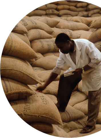
At the other end of the supply chain from finished goods inventory, a company might keep large stocks of parts and material inventory to meet variations in supplier deliveries. Inventory provides independence from vendors that a company does not have direct control over. Inventories of raw materials and purchased parts are kept on hand so that the production process will not be delayed as a result of missed or late deliveries or shortages from a supplier.
A company will purchase large amounts of inventory to take advantage of price discounts, as a hedge against anticipated price increases in the future, or because it can get a lower price by purchasing in volume. Walmart stores have been known to purchase a manufacturer's entire stock of soap powder or other retail item because they can get a very low price, which they subsequently pass on to their customers. Companies purchase large stocks of low-priced items when a supplier liquidates. In some cases, large orders will be made simply because the cost of ordering may be very high, and it is more cost-effective to have higher inventories than to order frequently.
Many companies find it necessary to maintain buffer inventories at different stages of their production process to provide independence between stages and to avoid work stoppages or delays. Inventories are kept between stages in the manufacturing process so that production can continue smoothly if there are temporary machine breakdowns or other work stoppages. Similarly, a stock of finished parts or products allows customer demand to be met in the event of a work stoppage or problem with transportation or distribution.
Inventory is kept between stages of a production process.
As we pointed out in previous chapters, information technology (IT) has become an enabler for effective supply chain management. Traditionally inventory was owned by the buyer (as opposed to the supplier), it was kept at the buyer's location, and the buyer controlled how and when its inventory was replenished. However, in recent years these traditional aspects of inventory management have changed, due in large part to advances in IT. Because of technology and software—including such IT tools as enterprises resource planning (ERP) systems (including forecasting software), barcodes, radio frequency identification (RFID, and point-of-sales data—companies can track and locate inventory throughout its supply chain, which enables them to locate inventory somewhere other than their own facility, and control it remotely or have someone else control it. These technologies have enabled modern supply chain management practices such as vendor managed inventory (VMI), continuous replenishment programs (CRP), supplier hubs, and outsourcing operations to third-party service providers (3PL). In these practices inventory can be located at the supplier's facility, at the buyer's, or somewhere in between. Unlike traditional practices, the supplier owns inventory until the buyer needs it and it is delivered, thus relieving the buyer of inventory costs; order sizes are reduced, deliveries (which the supplier pays for) are increased, and the buyer avoids maintaining storage facilities. However, for this to be effective the supplier must be able to minimize its own inventory costs and optimize its own supply chain, which can be achieved if the buyer shares end-use demand and sales data with its suppliers through IT. This enables suppliers to make replenishment decisions and provide inventory to the buyer, as it's needed. A recent supply chain management practice is for inventory to be located at "supplier hubs" that are usually at, or in very close proximity to, the buyer, and are often owned and operated by a 3PL provider, which shifts all responsibility and liability for inventory to the suppliers that share the hub. For a supplier hub to work, the supply chain members—buyers, suppliers, and 3PL providers—must share information through information technology. The 3PL provider uses information provided by the buyer and suppliers (including forecasts and sales data) to consolidate shipping among suppliers, plan and execute all logistics, connect and coordinate all supply chain members through an IT system, and operate the hub facility. Supplier hubs are being used successfully by such companies as Dell, Apple, Fiat, Hewlett-Packard, Nokia, Cisco, Sam's Club, Samsung, and Volkswagen.
Inventory must be sufficient to provide high-quality customer service in QM.
A company maintains inventory to meet its own demand and its customers' demand for items in the supply chain. The ability to meet effectively internal organizational demand or external customer demand in a timely, efficient manner is referred to as the level of customer service. A primary objective of supply chain management is to provide as high a level of customer service in terms of on-time delivery as possible. This is especially important in today's highly competitive business environment, where quality is such an important product characteristic. Customers for finished goods usually perceive quality service as availability of goods they want when they want them. (This is equally true of internal customers, such as company departments or employees.) To provide this level of quality customer service, the tendency is to maintain large stocks of all types of items. However, there is a cost associated with carrying items in inventory, which creates a cost tradeoff between the quality level of customer service and the cost of that service.
As the level of inventory increases to provide better customer service, inventory costs increase, whereas quality-related customer service costs, such as lost sales and loss of customers, decrease. The conventional approach to inventory management is to maintain a level of inventory that reflects a compromise between inventory costs and customer service. However, according to the contemporary "zero defects" philosophy of quality management, the long-term benefits of quality in terms of larger market share outweigh lower short-term production-related costs, such as inventory costs. Attempting to apply this philosophy to inventory management is not simple because one way of competing in today's diverse business environment is to reduce prices through reduced inventory costs.
Inventory is a stock of items kept by an organization to meet internal or external customer demand. Virtually every type of organization maintains some form of inventory. Department stores and grocery stores carry inventories of all the retail products they sell; a nursery has inventories of different plants, trees, and flowers; a rental-car agency has inventories of cars; and a major league baseball team maintains an inventory of players on its minor league teams. Even a family household maintains inventories of items such as food, clothing, medical supplies, and personal hygiene products.
Inventory: a stock of items kept to meet demand.
Most people think of inventory as a final product waiting to be sold to a retail customer—a new car or a can of tomatoes. This is certainly one of its most important uses. However, especially in a manufacturing firm, inventory can take on forms besides finished goods, including:
Raw materials
Purchased parts and supplies
Partially complete work in progress (WIP)
Items being transported
Tools, and equipment
Inventory management: how much and when to order.
The purpose of inventory management is to determine the amount of inventory to keep in stock—how much to order and when to replenish, or order. In this chapter we describe several different inventory systems and techniques for making these determinations.
The starting point for the management of inventory is customer demand. Inventory exists to meet customer demand. Customers can be inside the organization, such as a machine operator waiting for a part or partially completed product to work on. Customers can also be outside the organization—for example, an individual purchasing groceries or a new DVD player. In either case, an essential determinant of effective inventory management is an accurate forecast of demand. For this reason the topics of forecasting (Chapter 12) and inventory management are directly interrelated.
In general, the demand for items in inventory is either dependent or independent. Dependent demand items are typically component parts or materials used in the process of producing a final product. If an automobile company plans to produce 1000 new cars, then it will need 5000 wheels and tires (including spares). The demand for wheels is dependent on the production of cars—the demand for one item depends on demand for another item.
• Dependent demand: items are used internally to produce a final product.
Cars, retail items, grocery products, and office supplies are examples of independent demand items. Independent demand items are final or finished products that are not a function of, or dependent on, internal production activity. Independent demand is usually determined by external market conditions and, thus, is beyond the direct control of the organization. In this chapter we focus on the management of inventory for independent demand items.
• Independent demand: items are final products demanded by external customers.
Three basic costs are associated with inventory: carrying, or holding, costs; ordering costs; and shortage costs.
Inventory costs: carrying, ordering, and shortage
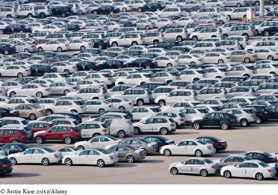
These offloaded cars at a port are an example of independent demand, as are appliances, computers, and houses. The tires on these cars are an example of an dependent demand item.
• Carrying costs: the costs of holding an item in inventory.
Carrying costs are the costs of holding items in inventory. Annual inventory carrying costs in the United States are estimated to be over $300 billion. These costs vary with the level of inventory in stock and occasionally with the length of time an item is held. That is, the greater the level of inventory over a period of time, the higher the carrying costs. In general, any cost that grows linearly with the number of units in stock is a carrying cost. Carrying costs can include the following items:
Facility storage (rent, depreciation, power, heat, cooling, lighting, security, refrigeration, taxes, insurance, etc.)
Material handling (equipment)
Labor
Record keeping
Borrowing to purchase inventory (interest on loans, taxes, insurance)
Product deterioration, spoilage, breakage, obsolescence, pilferage
Carrying costs can range from 10 to 40% of the value of a manufactured item.
Carrying costs are normally specified in one of two ways. The usual way is to assign total carrying costs, determined by summing all the individual costs just mentioned, on a perunit basis per time period, such as a month or year. In this form, carrying costs are commonly expressed as a perunit dollar amount on an annual basis; for example, $10 per unit per year. Alternatively, carrying costs are sometimes expressed as a percentage of the value of an item or as a percentage of average inventory value. It is generally estimated that carrying costs range from 10 to 40% of the value of a manufactured item.
• Ordering costs: the costs of replenishing inventory.
Ordering costs are the costs associated with replenishing the stock of inventory being held. These are normally expressed as a dollar amount per order and are independent of the order size. Annual ordering costs vary with the number of orders made—as the number of orders increases, the ordering cost increases. In general, any cost that increases linearly with the number of orders is an ordering cost. Costs incurred each time an order is made can include requisition and purchase orders, transportation and shipping, receiving, inspection, handling, and accounting and auditing costs.
Ordering costs react inversely to carrying costs. As the size of orders increases, fewer orders are required, reducing ordering costs. However, ordering larger amounts results in higher inventory levels and higher carrying costs. In general, as the order size increases, ordering costs decrease and carrying costs increase.
• Shortage costs: temporary or permanent loss of sales when demand cannot be met.
Shortage costs, also referred to as stockout costs, occur when customer demand cannot be met because of insufficient inventory. If these shortages result in a permanent loss of sales, shortage costs include the loss of profits. Shortages can also cause customer dissatisfaction and a loss of goodwill that can result in a permanent loss of customers and future sales. Some studies have shown that approximately 8% of shoppers will not find the product they want to purchase in stock, which will ultimately result in total lost sales of about 3%.
In some instances, the inability to meet customer demand or lateness in meeting demand results in penalties in the form of price discounts or rebates. When demand is internal, a shortage can cause work stoppages in the production process and create delays, resulting in downtime costs and the cost of lost production (including indirect and direct production costs).
Costs resulting from lost sales because demand cannot be met are more difficult to determine than carrying or ordering costs. Therefore, shortage costs are frequently subjective estimates and sometimes an educated guess.
Shortages occur because carrying inventory is costly. As a result, shortage costs have an inverse relationship to carrying costs—as the amount of inventory on hand increases, the carrying cost increases, whereas shortage costs decrease.
The objective of inventory management is to employ an inventory control system that will indicate how much should be ordered and when orders should take place so that the sum of the three inventory costs just described will be minimized.
An inventory system controls the level of inventory by determining how much to order (the level of replenishment) and when to order. There are two basic types of inventory systems: a continuous (or fixed-order-quantity) system and a periodic (or fixed-time-period) system. In a continuous system, an order is placed for the same constant amount whenever the inventory on hand decreases to a certain level, whereas in a periodic system, an order is placed for a variable amount after specific regular intervals.
In a continuous inventory system (also referred to as a perpetual system and a fixed-order-quantity system), a continual record of the inventory level for every item is maintained. Whenever the inventory on hand decreases to a predetermined level, referred to as the reorder point, a new order is placed to replenish the stock of inventory. The order that is placed is for a fixed amount that minimizes the total inventory costs. This amount, called the economic order quantity, is discussed in greater detail later.
• Continuous inventory system: a constant amount is ordered when inventory declines to a predetermined level.
A positive feature of a continuous system is that the inventory level is continuously monitored, so management always knows the inventory status. This is advantageous for critical items such as replacement parts or raw materials and supplies. However, maintaining a continual record of the amount of inventory on hand can also be costly.
A simple example of a continuous inventory system is a ledger-style checkbook that many of us use on a daily basis. Our checkbook comes with 300 checks; after the 200th check has been used (and there are 100 left), there is an order form for a new batch of checks. This form, when turned in at the bank, initiates an order for a new batch of 300 checks. Many office inventory systems use reorder cards that are placed within stacks of stationery or at the bottom of a case of pens or paper clips to signal when a new order should be placed. If you look behind the items on a hanging rack in a Kmart store, there will be a card indicating it is time to place an order for the item for an amount indicated on the card.
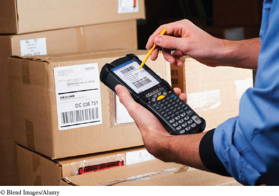
Continuous inventory systems often incorporate information technology tools to improve the speed and accuracy of data entry. A familiar example is the computerized checkout system with a laser scanner used by many supermarkets and retail stores. The laser scanner reads the universal product code (UPC), or bar code, from the product package; the transaction is instantly recorded, and the inventory level updated. Such a system is not only quick and accurate, it also provides management with continuously updated information on the status of inventory levels. Many manufacturing companies' suppliers and distributors also use bar code systems and handheld laser scanners to inventory materials, supplies, equipment, in-process parts, and finished goods.
To consumers the most familiar type of bar code scanners are used with cash registers at retail stores, where the bar code is a single line with 11 digits, the first 6 identifying a manufacturer and the last 5 assigned to a specific product by the manufacturer. This employee is using a portable hand held bar code scanner to scan a bar code for inventory control. In addition to identifying the product, it can indicate where a product came from, where it is supposed to go, and how the product should be handled in transit.
• Periodic inventory system: an order is placed for a variable amount after a fixed passage of time.
In a periodic inventory system (also referred to as a fixed-time-period system or a periodic review system), the inventory on hand is counted at specific time intervals—for example, every week or at the end of each month. After the inventory in stock is determined, an order is placed for an amount that will bring inventory back up to a desired level. In this system, the inventory level is not monitored at all during the time interval between orders, so it has the advantage of little or no required record keeping. The disadvantage is less direct control. This typically results in larger inventory levels for a periodic inventory system than in a continuous system to guard against unexpected stockouts early in the fixed period. Such a system also requires that a new order quantity be determined each time a periodic order is made.
An example of a periodic inventory system is a college or university bookstore. Textbooks are normally ordered according to a periodic system, wherein a count of textbooks in stock (for every course) is made after the first few weeks of a semester or quarter. An order for new textbooks for the next semester is then made according to estimated course enrollments for the next term (i.e., demand) and the amount remaining in stock. Smaller retail stores, drugstores, grocery stores, and offices sometimes use periodic systems—the stock level is checked every week or month, often by a vendor, to see how much should be ordered.
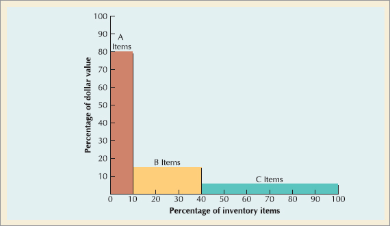
The ABC system is a method for classifying inventory according to several criteria, including its dollar value to the firm. Typically, thousands of independent demand items are held in inventory by a company, especially in manufacturing, but a small percentage is of such a high dollar value to warrant close inventory control. In general, about 5 to 15% of all inventory items account for 70 to 80% of the total dollar value of inventory. These are classified as A, or Class A, items. B items represent approximately 30% of total inventory units but only about 15% of total inventory dollar value. C items generally account for 50 to 60% of all inventory units but represent only 5 to 10% of total dollar value. For example, a discount store such as Walmart normally stocks a relatively small number of televisions, a somewhat larger number of bicycles or sets of sheets, and hundreds of boxes of soap powder, bottles of shampoo, and AA batteries. Figure 13.1 shows the approximate ABC classes.
• ABC system: an inventory classification system in which a small percentage of (A) items account for most of the inventory value.
In ABC analysis each class of inventory requires different levels of inventory monitoring and control—the higher the value of the inventory, the tighter the control. Class A items should experience tight inventory control; B and C require more relaxed (perhaps minimal) attention. However, the original rationale for ABC analysis was that continuous inventory monitoring was expensive and not justified for many items. The wide use of bar code scanners may have eroded that reasoning. At least for larger companies, bar codes have made continuous monitoring cheap enough to use for all item classes.
A items require close inventory control because of their high value; B and C items less control.
The first step in ABC analysis is to classify all inventory items as either A, B, or C. Each item is assigned a dollar value, which is computed by multiplying the dollar cost of one unit by the annual demand for that item. All items are then ranked according to their annual dollar value, with, for example, the top 10% classified as A items, the next 30% as B items, and the last 60% as C items. These classifications will not be exact, but they have been found to be close to the actual occurrence in firms with remarkable frequency.
A items require close inventory control because of their high value; B and C items less control.
The next step is to determine the level of inventory control for each classification. Class A items require tight inventory control because they represent such a large percentage of the total dollar value of inventory. These inventory levels should be as low as possible, and safety stocks minimized. This requires accurate demand forecasts and detailed record keeping. The appropriate inventory control system and inventory modeling procedure to determine order quantity should be applied. In addition, close attention should be given to purchasing policies and procedures if the inventory items are acquired from outside the firm. B and C items require less stringent inventory control. Since carrying costs are usually lower for C items, higher inventory levels can sometimes be maintained with larger safety stocks. It may not be necessary to control C items beyond simple observation. In general, A items frequently require a continuous control system, where the inventory level is continuously monitored; a periodic review system with less monitoring will suffice for C items.
Although cost is the predominant reason for inventory classification, other factors such as scarcity of parts or difficulty of supply may also be reasons for giving items a higher priority. For example, long lead times for some parts might be a problem for a company in Australia ordering from Europe, thus requiring a higher-priority classification for those parts.
In a continuous, or fixed-order-quantity, system when inventory reaches a specific level, referred to as the reorder point, a fixed amount is ordered. The most widely used and traditional means for determining how much to order in a continuous system is the economic order quantity (EOQ) model, also referred to as the economic lot-size model. The earliest published derivation of the basic EOQ model formula in 1915 is credited to Ford Harris, an employee at Westinghouse.
• Economic order quantity (EOQ): the optimal order quantity that will minimize total inventory costs.
The function of the EOQ model is to determine the optimal order size that minimizes total inventory costs. There are several variations of the EOQ model, depending on the assumptions made about the inventory system. We will describe two model versions: the basic EOQ model and the production quantity model.
Assumptions of EOQ model
The basic EOQ model is a formula for determining the optimal order size that minimizes the sum of carrying costs and ordering costs. The model formula is derived under a set of simplifying and restrictive assumptions, as follows:
Demand is known with certainty and is constant over time.
No shortages are allowed.
Lead time for the receipt of orders is constant.
The order quantity is received all at once.
• Order cycle: the time between receipt of orders in an inventory cycle.
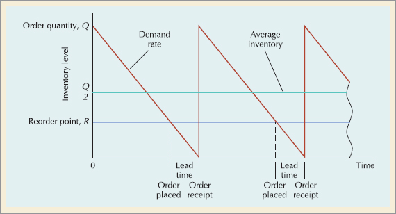
These basic model assumptions are reflected in Figure 13.2, which describes the continuous-inventory order cycle system inherent in the EOQ model. An order quantity, Q, is received and is used up over time at a constant rate. When the inventory level decreases to the reorder point, R, a new order is placed; a period of time, referred to as the lead time, is required for delivery. The order is received all at once just at the moment when demand depletes the entire stock of inventory—the inventory level reaches 0—so there will be no shortages. This cycle is repeated continuously for the same order quantity, reorder point, and lead time.
EOQ is a continuous inventory system.
As we mentioned, the economic order quantity is the order size that minimizes the sum of carrying costs and ordering costs. These two costs react inversely to each other. As the order size increases, fewer orders are required, causing the ordering cost to decline, whereas the average amount of inventory on hand will increase, resulting in an increase in carrying costs. Thus, in effect, the optimal order quantity represents a compromise between these two inversely related costs.
The total annual ordering cost is computed by multiplying the cost per order, designated as Co, times the number of orders per year. Since annual demand, D, is assumed to be known and to be constant, the number of orders will be D/Q, where Q is the order size and
The only variable in this equation is Q; both Co and D are constant parameters. Thus, the relative magnitude of the ordering cost is dependent on the order size.
Total annual carrying cost is computed by multiplying the annual per-unit carrying cost, designated as Cc, multiplied by the average inventory level. The average inventory level is one-half of Q or Q/2, as shown in Figure 13.2.
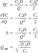
The total annual inventory cost is the sum of the ordering and carrying costs:
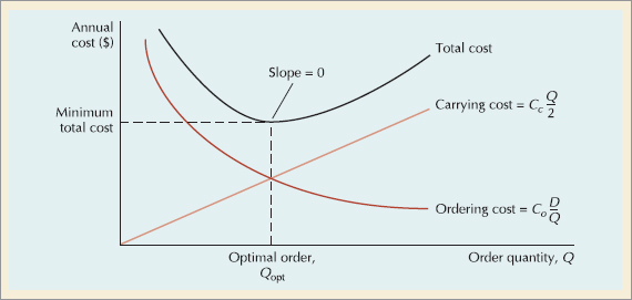
The graph in Figure 13.3 shows the inverse relationship between ordering cost and carrying cost, resulting in a convex total cost curve.
Optimal Q corresponds to the lowest point on the total cost curve.
The optimal order quantity occurs at the point in Figure 13.3 where the total cost curve is at a minimum, which coincides exactly with the point where the carrying cost curve intersects the ordering cost curve. This enables us to determine the optimal value of Q by equating the two cost functions and solving for Q:
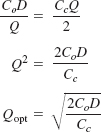
Alternatively, the optimal value of Q can be determined by differentiating the total cost curve with respect to Q, setting the resulting function equal to zero (the slope at the minimum point on the total cost curve), and solving for Q:
The total minimum cost is determined by substituting the value for the optimal order size, Qopt, into the total cost equation:
The Economic Order Quantity
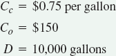
The ePaint Store stocks paint in its warehouse and sells it online on its Internet Web site. The store stocks several brands of paint; however, its biggest seller is Sharman-Wilson Ironcoat paint. The company wants to determine the optimal order size and total inventory cost for Ironcoat paint given an estimated annual demand of 10,000 gallons of paint, an annual carrying cost of $0.75 per gallon, and an ordering cost of $150 per order. They would also like to know the number of orders that will be made annually and the time between orders (i.e., the order cycle).
Solution
The optimal order size is
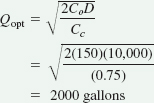
The total annual inventory cost is determined by substituting Qopt into the total cost formula:

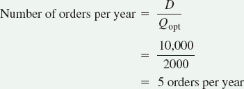
The number of orders per year is computed as follows:
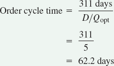
Given that the company processes orders 311 days annually (365 days minus 52 Sundays, Thanksgiving, and Christmas), the order cycle is
The optimal order quantity, determined in this example, and in general, is an approximate value, since it is based on estimates of carrying and ordering costs as well as uncertain demand (although all of these parameters are treated as known, certain values in the EOQ model). In practice it is desirable to round the Q values off to some nearby pragmatic value. The precision of a decimal place is generally not necessary. In addition, because the optimal order quantity is computed from a square root, errors or variations in the cost parameters and demand tend to be dampened. For instance, in Example 13.2, if the order cost had actually been 30% higher, or $200, the resulting optimal order size would have varied only by a little under 10% (i.e., 2190 gallons instead of 2000 gallons). Variations in both inventory costs will tend to offset each other, since they have an inverse relationship. As a result, the EOQ model is relatively resilient to errors in the cost estimates and demand, or is robust, which has tended to enhance its popularity.
The EOQ model is robust; because Q is a square root, errors in the estimation of D, Cc, and Co are dampened.
A variation of the basic EOQ model is the production quantity model, also referred to as the gradual usage and non-instantaneous receipt model. In this EOQ model the assumption that orders are received all at once is relaxed. The order quantity is received gradually over time, and the inventory level is depleted at the same time it is being replenished. This situation is commonly found when the inventory user is also the producer, as in a manufacturing operation where a part is produced to use in a larger assembly. This situation also can occur when orders are delivered continuously over time or when a retailer is also the producer.
• Production quantity model: an inventory system in which an order is received gradually, as inventory is simultaneously being depleted.
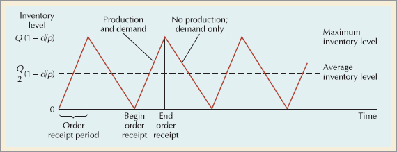
The noninstantaneous receipt model is shown graphically in Figure 13.4. The inventory level is gradually replenished as an order is received. In the basic EOQ model, average inventory was half the maximum inventory level, or Q/2, but in this model variation, the maximum inventory level is not simply Q; it is an amount somewhat lower than Q, adjusted for the fact the order quantity is depleted during the order receipt period.
Relaxing the assumption that Q is received all at once.
In order to determine the average inventory level, we define the following parameters unique to this model:
p = daily rate at which the order is received over time, also known as the production rate
d = the daily rate at which inventory is demanded
The demand rate cannot exceed the production rate, since we are still assuming that no shortages are possible, and, if d = p, there is no order size, since items are used as fast as they are produced. For this model the production rate must exceed the demand rate, or p ≥ d.
Observing Figure 13.4 we see that the time required to finish receiving an order is the order quantity divided by the rate at which the order is received, or Q/p. For example, if the order size is 100 units and the production rate, p, is 20 units per day, the order will be received over five days. The amount of inventory that will be depleted or used up during this time period is determined by multiplying by the demand rate: (Q/p)d. For example, if it takes five days to receive the order and during this time inventory is depleted at the rate of two units per day, then 10 units are used. As a result, the maximum amount of inventory on hand is the order size minus the amount depleted during the receipt period, computed as
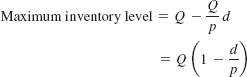
Since this is the maximum inventory level, the average inventory level is determined by dividing this amount by 2:
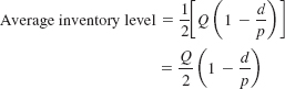
The total carrying cost using this function for average inventory is
In this case the ordering cost, Co, is often the setup cost for production.
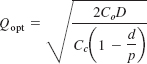
Thus, the total annual inventory cost is determined according to the following formula:
Solving this function for the optimal value Q,
The Production Quantity Model
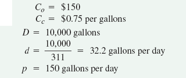
Assume that the ePaint Store has its own manufacturing facility in which it produces Ironcoat paint. The ordering cost, Co, is the cost of setting up the production process to make paint. Co = $150. Recall that Cc = $0.75 per gallon and D = 10,000 gallons per year. The manufacturing facility operates the same days the store is open (i.e., 311 days) and produces 150 gallons of paint per day. Determine the optimal order size, total inventory cost, the length of time to receive an order, the number of orders per year, and the maximum inventory level.
Solution
The optimal order size is determined as follows:

Although an order of 2256.8 gallons should be rounded to 2257, we will use the 2256.8 to compute total cost.
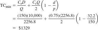
This value is substituted into the following formula to determine total minimum annual inventory cost:
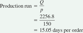
The length of time to receive an order for this type of manufacturing operation is commonly called the length of the production run.
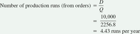
The number of orders per year is actually the number of production runs that will be made:
Finally, the maximum inventory level is
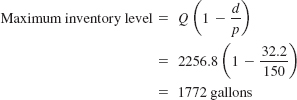
Thus, ePaint will need to set aside storage space sufficient to accommodate these 1772 gallons of paint.
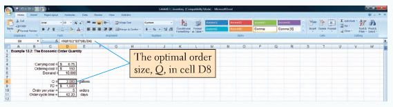
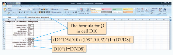
EOQ analysis can be done with Excel. The Excel solution screen for Example 13.2 is shown in Exhibit 13.1. The Excel screen for the production quantity model in Example 13.3 is shown in Exhibit 13.2.
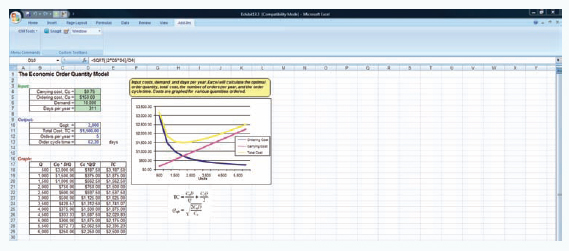
OM tools has modules to solve all the various inventory models illustrated in this chapter, including the ABC model for Example 13.1, the EOQ, and production quality models for Examples 13.2 and 13.3, the quantity discount model (Example 13.4), the recorder point model (Examples 13.5 and 13.6), and the fixed-period model (Example 13.7). As an example, Exhibit 13.3 shows the OM Tools spreadsheet for the EOQ Model in Example 13.2.
• Quantity Discount: given for specific higher order quantities.
A quantity discount is a price discount on an item if predetermined numbers of units are ordered. In the back of a magazine you might see an advertisement for a firm stating that it will produce a coffee mug (or hat) with a company or organizational logo on it, and the price will be $5 per mug if you purchase 100, $4 per mug if you purchase 200, or $3 per mug if you purchase 500 or more. Many manufacturing companies receive price discounts for ordering materials and supplies in high volume, and retail stores receive price discounts for ordering merchandise in large quantities.
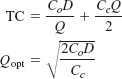
The basic EOQ model can be used to determine the optimal order size with quantity discounts; however, the application of the model is slightly altered. The total inventory cost function must now include the purchase price of the item being ordered:
Determining if an order size with a discount is more cost effective than optimal Q.
where
P = per-unit price of the item
D = annual demand
Purchase price was not considered as part of our basic EOQ formulation earlier because it had no impact on the optimal order size. In the preceding formula PD is a constant value that would not alter the basic shape of the total cost curve; that is, the minimum point on the cost curve would still be at the same location, corresponding to the same value of Q. Thus, the optimal order size is the same no matter what the purchase price is. However, when a discount price is available, it is associated with a specific order size, which may be different from the optimal order size, and the customer must evaluate the tradeoff between possibly higher carrying costs with the discount quantity versus EOQ cost. As a result, the purchase price does affect the order-size decision when a discount is available.
The EOQ cost model with constant carrying costs for a pricing schedule with two discounts, d1 and d2, is illustrated in Figure 13.5 for the following discounts:

Notice in Figure 13.5 that the optimal order size, Qopt, is the same regardless of the discount price. Although the total cost curve decreases with each discount in price (i.e., d1 and d2), since ordering and carrying cost are constant, the optimal order size, Qopt, does not change.
The graph in Figure 13.5 reflects the composition of the total cost curve resulting from the discounts kicking in at two successively higher order quantities. The first segment of the total cost curve (with no discount) is valid only up to 99 units ordered. Beyond that quantity, the total cost curve (represented by the topmost dashed line) is meaningless because above 100 units there is a discount (d1). Between 100 and 199 units the total cost drops down to the middle curve. This middle-level cost curve is valid only up to 199 units because at 200 units there is another, lower discount (d2). So the total cost curve has two discrete steps, starting with the original total cost curve, dropping down to the next level cost curve for the first discount, and finally dropping to the third-level cost curve for the final discount.
Notice that the optimal order size, Qopt, is feasible only for the middle level of the total cost curve, TC(d1)—it does not coincide with the top level of the cost curve, TC, or the lowest level, TC(d2). If the optimal EOQ order size had coincided with the lowest level of the total cost curve, TC(d2), it would have been optimal order size for the entire discount price schedule. Since it does not coincide with the lowest level of the total cost curve, the total cost with Qopt must be compared to the lower-level total cost using Q(d2) to see which results in the minimum total cost. In this case the optimal order size is 200.
A Quantity Discount with Constant Carrying Cost
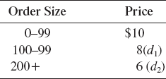
Avtek, a distributor of audio and video equipment, wants to reduce a large stock of televisions. It has offered a local chain of stores a quantity discount pricing schedule, as follows:
Quantity | Price |
|---|---|
1–49 | $1400 |
50–89 | 1100 |
90+ | 900 |
The annual carrying cost for the stores for a TV is $190, the ordering cost is $2,500, and annual demand for this particular model TV is estimated to be 200 units. The chain wants to determine if it should take advantage of this discount or order the basic EOQ order size.
Solution
First determine the optimal order size and total cost with the basic EOQ model.
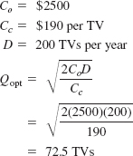
Although we will use Qopt = 72.5 in the subsequent computations, realistically the order size would be 73 televisions. This order size is eligible for the first discount of $1100; therefore, this price is used to compute total cost:
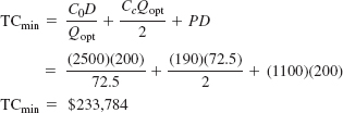
Since there is a discount for a larger order size than 50 units (i.e., there is a lower cost curve), this total cost of $233,784 must be compared with total cost with an order size of 90 and a discounted price of $900:
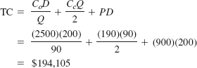
Since this total cost is lower ($194,105 < $233,784), the maximum discount price should be taken, and 90 units should be ordered. We know that there is no order size larger than 90 that would result in a lower cost, since the minimum point on this total cost curve has already been determined to be 73.
It is also possible to use Excel to solve the quantity-discount model with constant carrying cost. Exhibit 13.4 shows the Excel solution screen for Example 13.4. Notice that the selection of the appropriate order size, Q, that results in the minimum total cost for each discount range is determined by the formulas embedded in cells, E8, E9, and E10. For example, the formula for the first quantity-discount range, "1–49," is embedded in cell E8 and shown on the formula bar at the top of the screen, "=IF(D8.=B8, D8, B8)." This means that if the discount order size in cell D8 (i.e., Q = 72.55) is greater than or equal to the quantity in cell B8 (i.e., 1), then the quantity in cell D8 (72.55) is selected; otherwise the amount in cell B8 is selected. The formulas in cells E9 and E10 are constructed similarly. The result is that the order quantity for the final discount range, Q = 90, is selected.

In our description of the EOQ models in the previous sections, we addressed how much should be ordered. Now we will discuss the other aspect of inventory management, when to order. The determinant of when to order in a continuous inventory system is the reorder point, the inventory level at which a new order is placed.
• Reorder point: the level of inventory at which a new order should be placed.
The reorder point for our basic EOQ model with constant demand and a constant lead time to receive an order is equal to the amount demanded during the lead time,
R = dL
where
d = demand rate per period (e.g., daily)
L = lead time
Reorder Point for the Basic EOQ Model
The ePaint Internet Store in Example 13.2 is open 311 days per year. If annual demand is 10,000 gallons of Ironcoat paint and the lead time to receive an order is 10 days, determine the reorder point for paint.
Solution
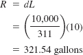
When the inventory level falls to approximately 321 gallons of paint, a new order is placed. Notice that the reorder point is not related to the optimal order quantity or any of the inventory costs.
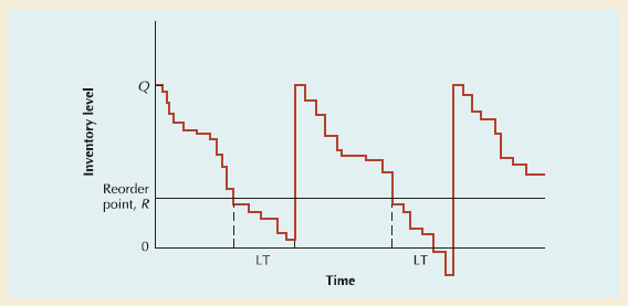
In Example 13.5, an order is made when the inventory level reaches the reorder point. During the lead time, the remaining inventory in stock will be depleted at a constant demand rate, such that the new order quantity will arrive at exactly the same moment as the inventory level reaches zero. Realistically, demand—and, to a lesser extent lead time—are uncertain. The inventory level might be depleted at a faster rate during lead time. This is depicted in Figure 13.6 for uncertain demand and a constant lead time.
• Stockout: an inventory shortage.
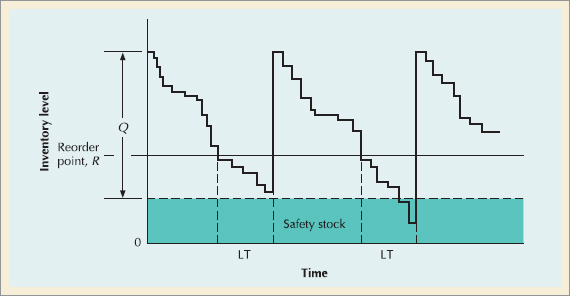
• Safety stock: a buffer added to the inventory on hand during lead time.
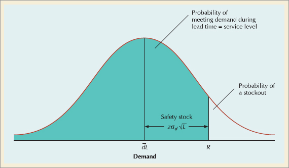
Notice in the second order cycle that a stockout occurs when demand exceeds the available inventory in stock. As a hedge against stockouts when demand is uncertain, a safety stock of inventory is frequently added to the expected demand during lead time. The addition of a safety stock to the stockout occurrence shown in Figure 13.6 is displayed in Figure 13.7.
There are several ways to determine the amount of the safety stock. One popular method is to establish a safety stock that will meet a specified service level. The service level is the probability that the amount of inventory on hand during the lead time is sufficient to meet expected demand— that is, the probability that a stockout will not occur. The term service is used, since the higher the probability that inventory will be on hand, the more likely that customer demand will be met—that is, that the customer can be served. A service level of 90% means that there is a 0.90 probability that demand will be met during the lead time, and the probability that a stockout will occur is 10%. The service level is typically a policy decision based on a number of factors, including carrying costs for the extra safety stock and lost sales if customer demand cannot be met.
• Service level: the probability that the inventory available during lead time will meet demand.
To compute the reorder point with a safety stock that will meet a specific service level, we will assume the demand during each day of lead time is uncertain, independent, and can be described by a normal distribution. The average demand for the lead time is the sum of the average daily demand for the days of the lead time, which is also the product of the average daily demands multiplied by the lead time. Similarly, the variance of the distribution is the sum of the daily variances for the number of days in the lead time. Using these parameters, we can compute the reorder point to meet a specific service level as
where
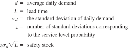
The term

The reorder point relative to the service level is shown in Figure 13.8. The service level is the shaded area, or probability, to the left of the reorder point, R.
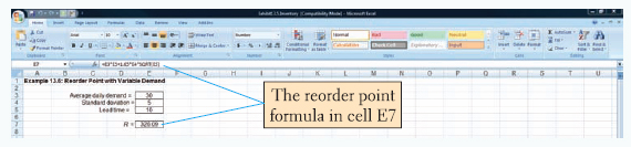
Reorder Point for Variable Demand
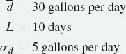
For the ePaint Internet Store in Example 13.2, we will assume that daily demand for Ironcoat paint is normally distributed with an average daily demand of 30 gallons and a standard deviation of 5 gallons of paint per day. The lead time for receiving a new order of paint is 10 days. Determine the reorder point and safety stock if the store wants a service level of 95%—that is, the probability of a stockout is 5%.
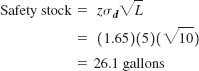
Solution
For a 95% service level, the value of z (from the Normal table in Appendix A) is 1.65. The safety stock is:
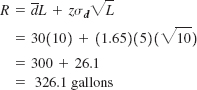
The reorder point is computed as follows:
Excel can be used to determine the reorder point for variable demand. Exhibit 13.5 shows the Excel screen for Example 13.6. Notice that the reorder point is computed using the formula in cell E7, which is shown on the formula bar at the top of the screen.
We defined a continuous, or fixed-order-quantity, inventory system as one in which the order quantity was constant and the time between orders varied. So far this type of inventory system has been the focus of our discussion. The less common periodic, or fixed-time-period, inventory system is one in which the time between orders is constant and the order size varies. Small retailers often use this sytem. Drugstores are one example of a business that sometimes uses a fixed-period inventory system. Drugstores stock a number of personal hygiene- and health-related products such as shampoo, toothpaste, soap, bandages, cough medicine, and aspirin.
Normally, the vendors who provide these items to the store will make periodic visits—every few weeks or every month—and count the stock of inventory on hand for their product. If the inventory is exhausted or at some predetermined reorder point, a new order will be placed for an amount that will bring the inventory level back up to the desired level. The drugstore managers will generally not monitor the inventory level between vendor visits but instead will rely on the vendor to take inventory.
Under this system, the vendor would bundle many small, low-cost items into a single order and delivery thereby saving costs. Since the items are generally of low value, larger safety stocks will not pose a significant cost. Also, if the items are noncritical, even if there is a stockout, it is not a big deal. However, inventory might be exhausted early in the time period between visits, resulting in a stockout that will not be remedied until the next scheduled order. As a result, a larger safety stock for more critical items is sometimes required for the fixed-interval system.
A periodic inventory system normally requires a larger safety stock.
If the demand rate and lead time are constant, then the fixed-period model will have a fixed-order quantity that will be made at specified time intervals, which is the same as the fixed-quantity (EOQ) model under similar conditions. However, as we have already explained, the fixed-period model reacts differently than the fixed-order model when demand is a variable.
The order size for a fixed-period model given variable daily demand that is normally distributed is determined by
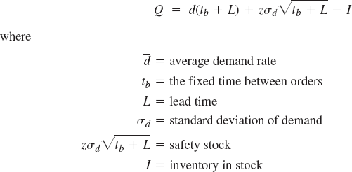
The first term in this formula,
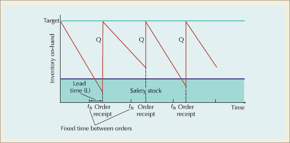
Figure 13.9 shows a periodic inventory system in which variable order sizes (Q) are placed at fixed time intervals (tb), and Example 13.7 on the following page illustrates this system.
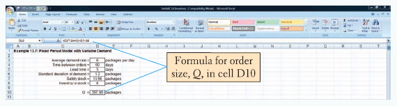
The order quantity for the fixed-period model with variable demand can be determined using Excel. The Excel screen for Example 13.7 is shown in Exhibit 13.6. Notice that the order quantity in cell D10 is computed with the formula shown on the formula bar at the top of the screen.
Order Size for Fixed-Period Model with Variable Demand
The KVS Pharmacy stocks a popular brand of over-the-counter flu and cold medicine. The average demand for the medicine is 6 packages per day, with a standard deviation of 1.2 packages. A vendor for the pharmaceutical company checks KVS's stock every 60 days. During one visit the store had 8 packages in stock. The lead time to receive an order is 5 days. Determine the order size for this order period that will enable KVS to maintain a 95% service level.
Solution
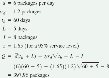
This will be rounded to 398 packages, or perhaps 400 if it is shipped in boxes of 100 packages.
The two types of systems for managing inventory are continuous and periodic, and we presented several models for determining how much to order and when to order for each system. However, we focused our attention primarily on the more commonly used continuous, fixed-order-quantity systems with EOQ models for determining order size and reorder points for determining when to order.
The objective of these order quantity models is to determine the optimal tradeoff between inventory carrying costs and ordering costs that would minimize total inventory cost. However, a drawback of approaching inventory management in this manner is that it can delude management into thinking that if they determine the minimum cost order quantity, they have achieved all they can in reducing inventory costs, which is not the case. Management should continually strive both to accurately assess and to reduce individual inventory costs. If management has accurately determined carrying and order costs, then they can seek ways to lower them that will reduce overall inventory costs regardless of the order size and reorder point.
Basic EOQ Model
EOQ Model with Noninstantaneous Receipt
Inventory Cost for Quantity Discounts
Reorder Point with Constant Demand and Lead Time
R = dL
Reorder Point with Variable Demand
Fixed-Time-Period Order Quantity with Variable Demand
ABC system a method for classifying inventory items according to their dollar value to the firm based on the principle that only a few items account for the greatest dollar value of total inventory.
carrying costs the cost of holding an item in inventory, including lost opportunity costs, storage, rent, cooling, lighting, interest on loans, and so on.
continuous inventory system a system in which the inventory level is continually monitored; when it decreases to a certain level, the reorder point, a fixed amount is ordered.
dependent demand typically, component parts or materials used in the process to produce a final product.
economic order quantity (EOQ) a fixed-order quantity that minimizes total inventory costs.
fixed-time-period system also known as a periodic system; an inventory system in which a variable amount is ordered after a predetermined, constant passage of time.
independent demand final or finished products whose demand is not a function of, or dependent on, internal production activity.
inventory a stock of items kept by an organization to meet internal or external customer demand.
order cycle the time between the receipt of orders in an inventory system.
ordering costs the cost of replenishing the stock of inventory including requisition cost, transportation and shipping, receiving, inspection, handling, and so forth.
periodic inventory system a system in which the inventory level is checked after a specific time period and a variable amount is ordered, depending on the inventory in stock.
production quantity model also known as the production lot-size model; an inventory system in which an order is received gradually and the inventory level is depleted at the same time it is being replenished.
quantity discount a pricing schedule in which lower prices are provided for specific (higher) order quantities.
reorder point a level of inventory in stock at which a new order is placed.
safety stock an amount added to the expected amount demanded during the lead time (the reorder point level) as a hedge against a stockout.
service level the probability that the amount of inventory on hand during the lead time is sufficient to meet expected demand.
shortage costs temporary or permanent loss of sales that will result when customer demand cannot be met.
stockout an inventory shortage occurring when demand exceeds the inventory in stock.
1. BASIC EOQ MODEL
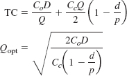
Electronic Village stocks and sells a particular brand of personal computer. It costs the store $450 each time it places an order with the manufacturer for the personal computers. The annual cost of carrying the PCs in inventory is $170. The store manager estimates that annual demand for the PCs will be 1200 units. Determine the optimal order quantity and the total minimum inventory cost.
SOLUTION
2. PRODUCTION QUANTITY MODEL
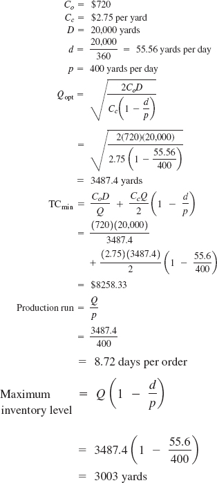
I-75 Discount Carpets manufactures Cascade carpet, which it sells in its adjoining showroom store near the interstate. Estimated annual demand is 20,000 yards of carpet with an annual carrying cost of $2.75 per yard. The manufacturing facility operates the same 360 days the store is open and produces 400 yards of carpet per day. The cost of setting up the manufacturing process for a production run is $720. Determine the optimal order size, total inventory cost, length of time to receive an order, and maximum inventory level.
SOLUTION
3. QUANTITY DISCOUNT
A manufacturing firm has been offered a particular component part it uses according to the following discount pricing schedule provided by the supplier.
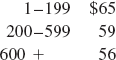
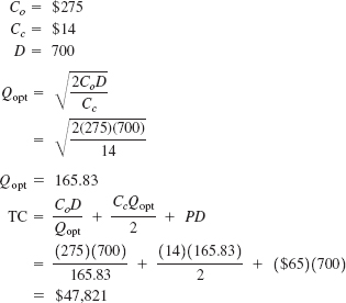
The manufacturing company uses 700 of the components annually, the annual carrying cost is $14 per unit, and the ordering cost is $275. Determine the amount the firm should order.
SOLUTION
First, determine the optimal order size and total cost with the basic EOQ model.
Next, compare the order size with the second-level quantity discount with an order size of 200 and a discount price of $59.
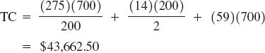
This discount results in a lower cost.
Finally, compare the current discounted order size with the fixed-price discount for Q = 600.
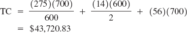
Since this total cost is higher, the optimal order size is 200 with a total cost of $43,662.50.
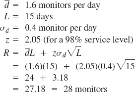
4. REORDER POINT WITH VARIABLE DEMAND
A computer products store stocks color graphics monitors, and the daily demand is normally distributed with a mean of 1.6 monitors and a standard deviation of 0.4 monitor. The lead time to receive an order from the manufacturer is 15 days. Determine the reorder point that will achieve a 98% service level.
SOLUTION
13-1. Describe the difference between independent and dependent demand and give an example of each for a pizza restaurant such as Domino's or Pizza Hut.
13-2. Distinguish between a fixed-order-quantity system and fixed-time-period system and give an example of each.
13-3. Discuss customer service level for an inventory system within the context of quality management.
13-4. Explain the ABC inventory classification system and indicate its advantages.
13-5. Identify the two basic decisions addressed by inventory management and discuss why the responses to these decisions differ for continuous and periodic inventory systems.
13-6. Describe the major cost categories used in inventory analysis and their functional relationship to each other.
13-7. Explain how the order quantity is determined using the basic EOQ model.
13-8. What are the assumptions of the basic EOQ model, and to what extent do they limit the usefulness of the model?
13-9. How are the reorder point and lead time related in inventory analysis?
13-10. Describe how the production quantity model differs from the basic EOQ model.
13-11. How must the application of the basic EOQ model be altered in order to reflect quantity discounts?
13-12. Why do the basic EOQ model variations not include the price of an item?
13-13. In the production quantity EOQ model, what would be the effect of the production rate becoming increasingly large as the demand rate became increasingly small, until the ratio d/p was negligible?
13-14. Explain in general terms how a safety stock level is determined using customer service level.
13-1. AV City stocks and sells a particular brand of laptop. It costs the firm $625 each time it places an order with the manufacturer for the laptops. The cost of carrying one laptop in inventory for a year is $130. The store manager estimates that total annual demand for the laptops will be 1500 units, with a constant demand rate throughout the year. Orders are received within minutes after placement from a local warehouse maintained by the manufacturer. The store policy is never to have stockouts of the laptops. The store is open for business every day of the year except Christmas Day. Determine the following:
Optimal order quantity per order
Minimum total annual inventory costs
The number of orders per year
The time between orders (in working days)
13-2. AV City (Problem 13-1) assumed with certainty that the ordering cost is $625/order and the inventory carrying cost is $130/unit/year. However, the inventory model parameters are frequently only estimates that are subject to some degree of uncertainty. Consider four cases of variation in the model parameters as follows: (a) Both ordering cost and carrying cost are 10% less than originally estimated; (b) both ordering cost and carrying cost are 10% higher than originally estimated; (c) ordering cost is 10% higher and carrying cost is 10% lower than originally estimated; and (d) ordering cost is 10% lower and carrying cost is 10% higher than originally estimated. Determine the optimal order quantity and total inventory cost for each of the four cases. Prepare a table with values from all four cases and compare the sensitivity of the model solution to changes in parameter values.
13-3. A firm is faced with the attractive situation in which it can obtain immediate delivery of an item it stocks for retail sale. The firm has therefore not bothered to order the item in any systematic way. However, recently profits have been squeezed due to increasing competitive pressures, and the firm has retained a management consultant to study its inventory management. The consultant has determined that the various costs associated with making an order for the item stocked are approximately $70 per order. She has also determined that the costs of carrying the item in inventory amount to approximately $27 per unit per year (primarily direct storage costs and forgone profit on investment in inventory). Demand for the item is reasonably constant over time, and the forecast is for 16,500 units per year. When an order is placed for the item, the entire order is immediately delivered to the firm by the supplier. The firm operates 6 days a week plus a few Sundays, or approximately 320 days per year. Determine the following:
Optimal order quantity per order
Total annual inventory costs
Optimal number of orders to place per year
Number of operating days between orders, based on the optimal ordering
13-4. The Sofaworld Company purchases upholstery material from Barrett Textiles. The company uses 45,000 yards of material per year to make sofas. The cost of ordering material from the textile company is $1,500 per order. It costs Sofaworld $0.70 per yard annually to hold a yard of material in inventory. Determine the optimal number of yards of material Sofaworld should order, the minimum total inventory cost, the optimal number of orders per year, and the optimal time between orders.
13-5. The Wallace Stationary Company purchases paper from the Seaboard Paper Company. Wallace produces stationary that require 1,415,000 sq. yards of stationary per year. The cost per order for the company is $2,200; the cost of holding 1 yard of paper in inventory is $0.08 per year. Determine the following:
Economic order quantity
Minimum total annual cost
Optimal number of orders per year
Optimal time between orders
13-6. The Ambrosia Bakery makes cakes for freezing and subsequent sale. The bakery, which operates five days a week, 52 weeks a year, can produce cakes at the rate of 116 cakes per day. The bakery sets up the cake-production operation and produces until a predetermined number (Q) have been produced. When not producing cakes, the bakery uses its personnel and facilities for producing other bakery items. The setup cost for a production run of cakes is $700. The cost of holding frozen cakes in storage is $9 per cake per year. The annual demand for frozen cakes, which is constant over time, is 6000 cakes. Determine the following:
Optimal production run quantity (Q)
Total annual inventory costs
Optimal number of production runs per year
Optimal cycle time (time between run starts)
Run length in working days
13-7. The EastCoasters Bicycle Shop operates 364 days a year, closing only on Christmas Day. The shop pays $300 for a particular bicycle purchased from the manufacturer. The annual holding cost per bicycle is estimated to be 25% of the dollar value of inventory. The shop sells an average of 18 bikes per week. The ordering cost for each order is $250. Determine the optimal order quantity and the total minimum cost.
13-8. The Chemco Company uses a highly toxic chemical in one of its manufacturing processes. It must have the product delivered by special cargo trucks designed for safe shipment of chemicals. As such, ordering (and delivery) costs are relatively high, at $3600 per order. The chemical product is packaged in 1-gallon plastic containers. The cost of holding the chemical in storage is $50 per gallon per year. The annual demand for the chemical, which is constant over time, is 7,000 gallons per year. The lead time from time of order placement until receipt is 10 days. The company operates 310 working days per year. Compute the optimal order quantity, total minimum inventory cost, and the reorder point.
13-9. The Food Place Supermarket stocks Munchkin Cookies. Demand for Munchkins is 5000 boxes per year (365 days). It costs the store $80 per order of Munchkins, and it costs $0.50 per box per year to keep the cookies in stock. Once an order for Munchkins is placed, it takes four days to receive the order from a food distributor. Determine the following:
Optimal order size
Minimum total annual inventory cost
Reorder point
13-10. Kroft Foods makes cheese to supply to stores in its area. The dairy can make 350 pounds of cheese per day, and the demand at area stores is 205 pounds per day. Each time the dairy makes cheese, it costs $175 to set up the production process. The annual cost of carrying a pound of cheese in a refrigerated storage area is $12. Determine the optimal order size and the minimum total annual inventory cost.
13-11. The Shotz Brewery produces an ale, which it stores in barrels in its warehouse and supplies to its distributors on demand. The demand for ale is 1800 barrels per day. The brewery can produce 3000 barrels per day. It costs $7500 to set up a production run for ale. Once it is brewed, the ale is stored in a refrigerated warehouse at an annual cost of $60 per barrel. Determine the economic order quantity and the minimum total annual inventory cost.
13-12. The purchasing manager for the Pacific Steel Company must determine a policy for ordering coal to operate 12 converters. Each converter requires exactly 5 tons of coal per day to operate, and the firm operates 360 days per year. The purchasing manager has determined that the ordering cost is $80 per order, and the cost of holding coal is 20% of the average dollar value of inventory held. The purchasing manager has negotiated a contract to obtain the coal for $12 per ton for the coming year.
Determine the optimal quantity of coal to receive in each order.
Determine the total inventory-related costs associated with the optimal ordering policy (do not include the cost of the coal).
If five days' lead time is required to receive an order of coal, how much coal should be on hand when an order is placed?
13-13. The TransCanada Lumber Company and Mill processes 10,000 logs annually, operating 250 days per year. Immediately upon receiving an order, the logging company's supplier begins delivery to the lumber mill at the rate of 60 logs per day. The lumber mill has determined that the ordering cost is $1600 per order, and the cost of carrying logs in inventory before they are processed is $15 per log on an annual basis. Determine the following:
The optimal order size
The total inventory cost associated with the optimal order quantity
The number of operating days between orders
The number of operating days required to receive an order
13-14. The Goodstone Tire Company produces a brand of tire called the Rainpath. The annual demand at its distribution center is 12,400 tires per year. The transport and handling costs are $2600 each time a shipment of tires is ordered at the distribution center. The annual carrying cost is $3.75 per tire.
Determine the optimal order quantity and the minimum total annual cost.
The company is thinking about relocating its distribution center, which would reduce transport and handling costs to $1900 per order but increase carrying costs to $4.50 per tire per year. Should the company relocate based on inventory costs?
13-15. The Deer Valley Farm produces a natural organic fertilizer, which it sells mostly to gardeners and homeowners. The annual demand for fertilizer is 220,000 pounds. The farm is able to produce 305,000 pounds annually. The cost to transport the fertilizer from the plant to the farm is $620 per load. The annual carrying cost is $0.12 per pound.
Compute the optimal order size, the maximum inventory level, and the total minimum cost.
If the farm can increase production capacity to 360,000 pounds per year, will it reduce total inventory cost?
13-16. Tradewinds Imports is an importer of ceramics from overseas. It has arranged to purchase a particular type of ceramic pottery from a Korean artisan. The artisan makes the pottery in 120-unit batches and will ship only that exact amount. The transportation and handling cost of a shipment is $7600 (not including the unit cost). The importer estimates its annual demand to be 1400 units. What storage and handling cost per unit does it need to achieve in order to minimize its inventory cost?
13-17. The KVS Pharmacy is open from 10:00 a.m. to 8:00 p.m., and it receives 200 calls per day for delivery orders. It costs the pharmacy $25 to send out its cars to make deliveries. The pharmacy estimates that each minute a customer spends waiting for their order costs the pharmacy $0.20 in lost sales.
How frequently should KVS send out its delivery cars each day? Indicate the total daily cost of deliveries.
If a car could only carry six orders how often would deliveries be made and what would be the cost?
13-18. The Olde Town Microbrewery makes Townside beer, which it bottles and sells in its adjoining restaurant and by the case. It costs $1700 to set up, brew, and bottle a batch of the beer. The annual cost to store the beer in inventory is $1.25 per bottle. The annual demand for the beer is 21,000 bottles and the brewery has the capacity to produce 30,000 bottles annually.
Determine the optimal order quantity, total annual inventory cost, the number of production runs per year, and the maximum inventory level.
If the microbrewery has only enough storage space to hold a maximum of 2500 bottles of beer in inventory, how will that affect total inventory costs?
13-19. JAL Trading is a Hong Kong manufacturer of electronic components. During the course of a year it requires container cargo space on ships leaving Hong Kong bound for the United States, Mexico, South America, and Canada. The company needs 280,000 cubic feet of cargo space annually. The cost of reserving cargo space is $7000 and the cost of holding cargo space is $0.80/ft3. Determine how much storage space the company should optimally order, the total cost, and how many times per year it should place an order to reserve space.
13-20. County Hospital orders syringes from a hospital supply firm. The hospital expects to use 40,000 per year. The cost to order and have the syringes delivered is $800. The annual carrying cost is $1.90 per syringe because of security and theft. The hospital supply firm offers the following quantity discount pricing schedule.
Quantity | Price |
|---|---|
0–999 | $3.40 |
10,000–19,999 | 3.20 |
20,000–29,999 | 3.00 |
30,000–39,999 | 2.80 |
40,000–49,999 | 2.60 |
50,000+ | 2.40 |
Determine the order size for the hospital.
13-21. The Interstate Carpet Discount Store has annual demand of 10,000 yards of Super Shag carpet. The annual carrying cost for a yard of this carpet is $1.25, and the ordering cost is $300. The carpet manufacturer normally charges the store $8 per yard for the carpet. However, the manufacturer has offered a discount price of $6.50 per yard if the store will order 5000 yards. How much should the store order, and what will be the total annual inventory cost for that order quantity?
13-22. Kelly's Tavern buys Shamrock draft beer by the keg from a local distributor. The bar has an annual demand of 900 kegs, which it purchases at a price of $60 per keg. The annual carrying cost is $7.20, and the cost per order is $160. The distributor has offered the bar a reduced price of $52 per barrel if it will order a minimum of 300 barrels. Should the bar take the discount?
13-23. The bookstore at Tech purchases jackets emblazoned with the school name and logo from a vendor. The vendor sells the jackets to the store for $38 apiece. The cost to the bookstore for placing an order is $120, and the annual carrying cost is 25% of the cost of a jacket. The bookstore manager estimates that 1700 jackets will be sold during the year. The vendor has offered the bookstore the following volume discount schedule: The annual demand for cups is 2.3 million, the annual carrying cost per box of cups is $1.90, and ordering cost is $320. Determine the optimal order quantity and total annual inventory cost.
Order Size | Discount |
|---|---|
1–299 | 0% |
300–499 | 2% |
500–799 | 4% |
800+ | 5% |
What is the bookstore's optimal order quantity, given this quantity discount information?
13-24. Determine the optimal order quantity of jackets and total annual cost in Problem 13-23 if the carrying cost is a constant $8 per jacket per year.
13-25. The office manager for the Metro Life Insurance Company orders letterhead stationery from an office products firm in boxes of 500 sheets. The company uses 6500 boxes per year. Annual carrying costs are $3 per box, and ordering costs are $28. The following discount price schedule is provided by the office supply company:
Order Quantity (boxes) | Price per Box |
|---|---|
200–999 | $16 |
1000–2999 | 14 |
3000–5999 | 13 |
6000+ | 12 |
Determine the optimal order quantity and the total annual inventory cost.
13-26. Determine the optimal order quantity and total annual inventory cost for boxes of stationery in Problem 13-25 if the carrying cost is 20% of the price of a box of stationery.
13-27. The 21,000-seat Air East Arena houses the local professional ice hockey, basketball, indoor soccer, and arena football teams as well as various trade shows, wrestling and boxing matches, tractor pulls, and circuses. Arena vending annually sells large quantities of soft drinks and beer in plastic cups with the name of the arena and the various team logos on them. The local container cup manufacturer that supplies the cups in boxes of 100 has offered arena management the following discount price schedule for cups:
Order Quantity (boxes) | Price per Box |
|---|---|
2000–6999 | $47 |
7000–11,999 | 43 |
12,000–19,999 | 41 |
20,000+ | 38 |
The annual demand for cups is 2.3 million, the annual carrying cost per box of cups is $1.90, and ordering cost is $320. Determine the optimal order quantity and total annual inventory cost.
13-28. Determine the optimal order quantity and total annual inventory cost for cups in Problem 13-27 if the carrying cost is 5% of the price of a box of cups.
13-29. The amount of denim used daily by the Southwest Apparel Company in its manufacturing process to make jeans is normally distributed with an average of 4000 yards of denim and a standard deviation of 600 yards. The lead time required to receive an order of denim from the textile mill is a constant 7 days. Determine the safety stock and reorder point if the company wants to limit the probability of a stockout and work stoppage to 5%.
13-30. In Problem 13-29, what level of service would a safety stock of 2000 yards provide?
13-31. The Paramount Paper company produces paper from wood pulp ordered from a lumber products firm. The paper company's daily demand for wood pulp is normally distributed, with a mean of 9000 pounds and a standard deviation of 1900 pounds. Lead time is eight days. Determine the reorder point if the paper company wants to limit the probability of a stockout and work stoppage to 2%.
13-32. Kelly's Tavern serves Shamrock draft beer to its customers. The daily demand for beer is normally distributed, with an average of 20 gallons and a standard deviation of 4 gallons. The lead time required to receive an order of beer from the local distributor is 12 days. Determine the safety stock and reorder point if the restaurant wants to maintain a 90% service level. What would be the increase in the safety stock if a 95% service level were desired?
13-33. The daily demand for Ironcoat paint at the Top Value Hardware Store in North Bay is normally distributed, with a mean of 30 gallons and a standard deviation of 10 gallons. The lead time for receiving an order of paint from the paint distributor is eight days. Since this is the only paint store in North Bay, the manager is interested in maintaining only a 75% service level. What reorder point should be used to meet this service level? The manager subsequently learned that a new paint store would open soon in North Bay, which has prompted her to increase the service level to 95%. What reorder point will maintain this service level?
13-34. IM Systems assembles microcomputers from generic components. It purchases its color monitors from a manufacturer in Taiwan; thus, there is a long lead time of 25 days. Daily demand is normally distributed with a mean of 3.5 monitors and a standard deviation of 1.2 monitors. Determine the safety stock and reorder point corresponding to a 90% service level.
13-35. IM Systems (Problem 13-34) is considering purchasing monitors from a U.S. manufacturer that would guarantee a lead time of eight days, instead of from the Taiwanese company. Determine the new reorder point given this lead time and identify the factors that would enter into the decision to change manufacturers.
13-36. KVS Pharmacy fills prescriptions for a popular children's antibiotic, Amoxycilin. The daily demand for Amoxycilin is normally distributed with a mean of 200 ounces and a standard deviation of 80 ounces. The vendor for the pharmaceutical firm that supplies the drug calls the drugstore's pharmacist every 30 days and checks the inventory of Amoxycilin. During a call the druggist indicated the store had 60 ounces of the antibiotic in stock. The lead time to receive an order is four days. Determine the order size that will enable the drugstore to maintain a 99% service level.
13-37. Food Place Market stocks frozen pizzas in a refrigerated display case. The average daily demand for the pizzas is normally distributed, with a mean of 8 pizzas and a standard deviation of 2.5 pizzas. A vendor for a packaged food distributor checks the market's inventory of frozen foods every 10 days; during a particular visit there were no pizzas in stock. The lead time to receive an order is three days. Determine the order size for this order period that will result in a 98% service level. During the vendor's following visit there were 5 frozen pizzas in stock. What is the order size for the next order period?
13-38. The Mediterranean Restaurant stocks a red Chilean table wine it purchases from a wine merchant in a nearby city. The daily demand for the wine at the restaurant is normally distributed, with a mean of 18 bottles and a standard deviation of 4 bottles. The wine merchant sends a representative to check the restaurant's wine cellar every 30 days, and during a recent visit there were 25 bottles in stock. The lead time to receive an order is two days. The restaurant manager has requested an order size that will enable him to limit the probability of a stockout to 5%.
13-39. The Aztec Company stocks a variety of parts and materials it uses in its manufacturing processes. Recently, as demand for its finished goods has increased, management has had difficulty managing parts inventory; they frequently run out of some crucial parts and seem to have an endless supply of others. In an effort to control inventory more effectively, they would like to classify their inventory of parts according to the ABC approach. Following is a list of selected parts and the annual usage and unit value for each:
Item Number | Annual Usage | Unit Cost |
|---|---|---|
1 | 36 | $350 |
2 | 510 | 30 |
3 | 50 | 23 |
4 | 300 | 45 |
5 | 18 | 1900 |
6 | 500 | 8 |
7 | 710 | 4 |
8 | 80 | 26 |
9 | 344 | 28 |
10 | 67 | 440 |
11 | 510 | 2 |
12 | 682 | 35 |
13 | 95 | 50 |
14 | 10 | 3 |
15 | 820 | 1 |
16 | 60 | $610 |
17 | 120 | 20 |
18 | 270 | 15 |
19 | 45 | 50 |
20 | 19 | 3200 |
21 | 910 | 3 |
22 | 12 | 4750 |
23 | 30 | 2710 |
24 | 24 | 1800 |
25 | 870 | 105 |
26 | 244 | 30 |
27 | 750 | 15 |
28 | 45 | 110 |
29 | 46 | 160 |
30 | 165 | 25 |
Classify the inventory items according to the ABC approach using dollar value of annual demand.
13-40. The EastCoasters Bicycle Shop stocks bikes; helmets; clothing; a variety of bike parts including chains, gears, tires, wheels; and biking accessories. The shop is in a storefront location on a busy street and it has very limited storage space for inventory. It often runs out of items and is unable to serve customers. To help manage its inventory the shop would like to classify the stock using the ABC system. Following is a list of items the shop stocks and the annual demand and unit value for each:
Item Number | Annual Usage | Unit Cost |
|---|---|---|
1 | 10 | $8 |
2 | 18 | 16 |
3 | 36 | 30 |
4 | 9 | 1230 |
5 | 4 | 760 |
6 | 3 | 810 |
7 | 19 | 420 |
8 | 56 | 35 |
9 | 105 | 17 |
10 | 27 | 350 |
11 | 19 | 36 |
12 | 12 | 115 |
13 | 7 | 2300 |
14 | 10 | 245 |
15 | 6 | 665 |
16 | 18 | 28 |
17 | 110 | $23 |
18 | 74 | 18 |
19 | 8 | 610 |
20 | 10 | 935 |
21 | 7 | 270 |
22 | 5 | 1400 |
23 | 5 | 900 |
24 | 46 | 67 |
25 | 32 | 160 |
26 | 101 | 45 |
27 | 83 | 12 |
28 | 54 | 16 |
29 | 14 | 42 |
30 | 9 | 705 |
31 | 7 | 37 |
32 | 16 | 26 |
Classify the inventory items according to the ABC approach using dollar value of annual demand.
13-41. Tara McCoy is the office administrator for the Department of Management at State University. The faculty uses a lot of printer paper and Tara is constantly reordering and frequently runs out. She orders the paper from the university central stores and several faculty have determined that the lead time to receive an order is normally distributed, with a mean of 2 days and a standard deviation of 0.5 day. The faculty have also determined that daily demand for the paper is normally distributed, with a mean of 2.6 packages and a standard deviation of 0.8 packages. What reorder point should Tara use in order not to run out 99% of the time?
13-42. The concession stand at the Shelby High School stadium sells slices of pizza during boys' and girls' soccer games. Concession stand sales are a primary source of revenue for the high school athletic programs, so the athletic director wants to sell as much food as possible; however, any pizza not sold is given away free to the players, coaches, and referees or it is thrown away. As such, the athletic director wants to determine a reorder point that will meet the demand for pizza. Pizza sales are normally distributed with a mean of 6 pizzas per hour and a standard deviation of 2.5 pizzas. The pizzas are ordered from Pizza Beth's restaurant, and the mean delivery time is 30 minutes, with a standard deviation of 8 minutes.
Currently the concession stand places an order when they have 1 pizza left. What level of service does this result in?
What should the reorder point be to have a 98% service level?
The Instant Paper Clip Office Supply Company
Christie Levine is the manager of the Instant Paper Clip Office Supply Company in Louisville. The company attempts to gain an advantage over its competitors by providing quality customer service, which includes prompt delivery of orders by truck or van and always being able to meet customer demand from its stock. In order to achieve this degree of customer service, it must stock a large volume of items on a daily basis at a central warehouse and at three retail stores in the city and suburbs. Christie maintains these inventory levels by borrowing cash on a daily basis from the First American Bank. She estimates that for the coming fiscal year the company's demand for cash to pay for inventory will be $17,000 per day for 305 working days. Any money she borrows during the year must be repaid with interest by the end of the year. The annual interest rate currently charged by the bank is 9%. Any time Christie takes out a loan to purchase inventory, the bank charges the company a loan origination fee of $1200 plus 2¼ points (2.25% of the amount borrowed).
Christie often uses EOQ analysis to determine optimal amounts of inventory to order for different office supplies. Now she is wondering if she can use the same type of analysis to determine an optimal borrowing policy. Determine the amount of the loan Christie should borrow from the bank, the total annual cost of the company's borrowing policy, and the number of loans the company should obtain during the year. Also determine the level of cash on hand at which the company should apply for a new loan given that it takes 15 days for a loan to be processed by the bank.
Suppose the bank offers Christie a discount as follows. On any loan amount equal to or greater than $500,000, the bank will lower the number of points charged on the loan origination fee from 2.25% to 2.00%. What would be the company's optimal amount borrowed?
The Texas Gladiators Apparel Store
The Texas Gladiators won the Super Bowl last year. As a result, sportswear such as hats, sweatshirts, sweat-pants, and jackets with the Gladiator's logo are popular. The Gladiators operate an apparel store outside the football stadium. It is near a busy highway, so the store has heavy customer traffic throughout the year, not just on game days. In addition, the stadium has high school or college football and soccer games almost every week in the fall, and baseball games in the spring and summer. The most popular single item the stadium store sells is a red and silver baseball-style cap with the Gladiators' logo on it. The cap has an elastic headband inside it, which conforms to different head sizes. However, the store has had a difficult time keeping the cap in stock, especially during the time between the placement and receipt of an order. Often customers come to the store just for the hat; when it is not in stock, customers are upset, and the store management believes they tend to go to other competing stores to purchase their Gladiators' clothing. To rectify this problem, the store manager, Jessica James, would like to develop an inventory control policy that would ensure that customers would be able to purchase the cap 99% of the time they asked for it. Jessica has accumulated the following demand data for the cap for a 30-week period. (Demand includes actual sales plus a record of the times a cap has been requested but not available and an estimate of the number of times a customer wanted a cap when it was not available but did not ask for it.)
The store purchases the hats from a small manufacturing company in Jamaica. The shipments from Jamaica are erratic, with a lead time of 20 days.
In the past, Ms. James has placed an order whenever the stock got down to 150 caps. What level of service does this reorder point correspond to? What would the reorder point and safety stock need to be to achieve the desired service level? Discuss how Jessica James might determine the order size of caps and what additional, if any, information would be needed to determine the order size.
Week | Demand |
|---|---|
1 | 38 |
2 | 51 |
3 | 25 |
4 | 60 |
5 | 35 |
6 | 42 |
7 | 29 |
8 | 46 |
9 | 55 |
10 | 19 |
11 | 28 |
12 | 41 |
13 | 37 |
14 | 44 |
15 | 45 |
16 | 56 |
17 | 62 |
18 | 53 |
19 | 46 |
20 | 41 |
21 | 52 |
22 | 38 |
23 | 49 |
24 | 46 |
25 | 47 |
26 | 41 |
27 | 39 |
28 | 50 |
29 | 28 |
30 | 34 |
Pharr Foods Company
Pharr Foods Company produces a variety of food products including a line of candies. One of its most popular candy items is "Far Stars," a bag of a dozen, individually wrapped, star-shaped candies made primarily from a blend of dark and milk chocolates, macadamia nuts, and a blend of heavy cream fillings. The item is relatively expensive, so Pharr Foods only produces it for its eastern market encompassing urban areas such as New York, Atlanta, Philadelphia, and Boston. The item is not sold in grocery or discount stores but mainly in specialty shops and specialty groceries, candy stores, and department stores. Pharr Foods supplies the candy to a single food distributor which has several warehouses on the East Coast. The candy is shipped in cases with 60 bags of the candy per case. Far Stars sell well despite the fact that they are expensive at $9.85 per bag (wholesale). Pharr uses highquality, fresh ingredients and does not store large stocks of the candy in inventory for very long periods of time.
Pharr's distributor believes that demand for the candy follows a seasonal pattern. It has collected demand data (i.e., cases sold) for Far Stars from its warehouses and the stores it supplies for the past three years, as follows.
Month | Demand (cases) | ||
|---|---|---|---|
Year 1 | Year 2 | Year 3 | |
January | 192 | 212 | 228 |
February | 210 | 223 | 231 |
March | 205 | 216 | 226 |
April | 260 | 252 | 293 |
May | 228 | 235 | 246 |
June | 172 | 220 | 229 |
July | 160 | 209 | 217 |
August | 147 | 231 | 226 |
September | 256 | 263 | 302 |
October | 342 | 370 | 410 |
November | 261 | 260 | 279 |
December | 273 | 277 | 293 |
The distributor must hold the candy inventory in climatecontrolled warehouses and be careful in handling it. The annual carrying cost is $116 per case. The item must be shipped a long distance from the manufacturer to the distributor. In order to keep the candy as fresh as possible, trucks must be air-conditioned and shipments must be direct, and are often less-than-truckload. As a result, ordering cost is $4700.
Pharr Foods makes Far Stars from three primary ingredients it orders from different suppliers: dark and milk chocolate, macadamia nuts, and, a special heavy cream filling. Except for its unique star shape, a Far Star is almost like a chocolate truffle. Each Far Star weighs 1.2 ounces and requires 0.70 ounce of blended chocolates, 0.50 ounce of macadamia nuts, and 0.40 ounce of filling to produce (including spillage and waste). Pharr Foods orders chocolate, nuts, and filling from its suppliers by the pound. The annual ordering cost is $5700 for chocolate, and the carrying cost is $0.45 per pound. The ordering cost for macadamia nuts is $6300, and the annual carrying cost is $0.63 per pound. The ordering cost for filling is $4500, and the annual average carrying cost is $0.55 per pound.
Each of the suppliers offers the candy manufacturer a quantity-discount price schedule for the ingredients as follows:
Chocolate | Macadamia Nuts | Filling | |||
|---|---|---|---|---|---|
Price | Quantity (lb) | Price | Quantity (lb) | Price | Quantity (lb) |
$3.05 | 0–50,000 | $6.50 | 0–30,000 | $1.50 | 0–40,000 |
2.90 | 50,001–100,000 | 6.25 | 30,001–70,000 | 1.35 | 40,001–80,000 |
2,75 | 100,001–150,000 | 5.95 | 70,000+ | 1.25 | 80,000+ |
2.60 | 150,000+ | ||||
Determine the inventory order quantity for Pharr's distributor. Compare the optimal order quantity with a seasonally adjusted forecast for demand. Does the order quantity seem adequate to meet the seasonal demand pattern for Far Stars? That is, is it likely that shortages or excessive inventories will occur? Can you identify the causes of the seasonal demand pattern for Far Stars? Determine the inventory order quantity for each of the three primary ingredients that Pharr Foods orders from its suppliers. Discuss the possible impact of the order policies of the food distributor and Pharr Foods on quality management and supply chain management.
Brown, R. G. Decision Rules for Inventory Management. New York: Holt, Rinehart and Winston, 1967.
Buchan, J., and E. Koenigsberg. Scientific Inventory Management. Upper Saddle River, N.J.: Prentice Hall, 1963.
Buffa, E. S., and Jefferey Miller. Production-Inventory Systems: Planning and Control, rev. ed. Homewood, IL: Irwin, 1979.
Churchman, C. W., R. L. Ackoff, and E. L. Arnoff. Introduction to Operations Research. New York: Wiley, 1957.
Fetter, R. B., and W. C. Dalleck. Decision Models for Inventory Management. Homewood, IL: Irwin, 1961.
Greene, J. H. Production and Inventory Control. Homewood, IL: Irwin, 1974.
Hadley, G., and T. M. Whitin. Analysis of Inventory Systems. Upper Saddle River, N.J.: Prentice Hall, 1963.
McGee, J. F., and D. M. Boodman. Production Planning and Inventory Control, 2nd ed. New York: McGraw-Hill, 1967.
Starr, M. K., and D. W. Miller. Inventory Control: Theory and Practice. Upper Saddle River, N.J.: Prentice Hall, 1962.
Wagner, H. M. Statistical Management of Inventory Systems. New York: Wiley, 1962.
Whitin, T. M. The Theory of Inventory Management. Princeton, N.J.: Princeton University Press, 1957.