3.6. Gradually Varied Flow

Search in book...
Toggle Font Controls
Create new playlist

Name your new playlist

Playlist description (optional)
Sign In

Email address

Password

Forgot Password?

or

Continue with Facebook

Continue with Google
Sign Up

Full Name

Email address

Confirm Email Address

Password

or

Continue with Facebook

Continue with Google

3.6. Gradually Varied Flow

The governing equation derived from the energy conservation law for describing the gradually varied flow is given by:

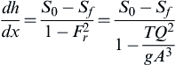$\frac{d h}{d x} = \frac{S_{0} - S_{f}}{1 - F_{r}^{2}} = \frac{S_{0} - S_{f}}{1 - \frac{T Q^{2}}{g A^{3}}}$ $\frac{d h}{d x} = \frac{S_{0} - S_{f}}{1 - F_{r}^{2}} = \frac{S_{0} - S_{f}}{1 - \frac{T Q^{2}}{g A^{3}}}$

(3.150)

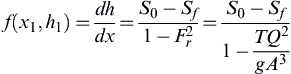
in which S₀ is the bottom slope of the channel, S_f is the friction or energy slope, F_r is the Froude number, dh/dx is the variation flow depth with respect to distance x, Q is the discharge (m³/s), T is top width of the channel (m), and A is the water area (m²).

3.6.1. Classification of Gradually Varied Flow

To classify gradually varied flow, first it is necessary to classify the slope, which is based on the relative magnitude of normal depth and critical depth of flow. The hydraulic classification of slopes following the subclassification of gradually varied flow is summarized in Table 3.9.

3.6.2. Computation of Gradually Varied Flow or Water Level Profile

Various procedures have been developed for determining the water surface profile in gradually varied flow (Henderson, 1966; US Army Corps of Engineers, 2002; Chaudhry, 2008). The computations are started at a location where the flow depth for specified discharge is known. When flow is subcritical, the flow profile is computed in the upstream direction, whereas the computations are made in the downstream direction when flow is supercritical. Among the various methods, some of the commonly used methods will be described here.

Table 3.9

Classification of Gradually Varied Flow

Slope Class	Type	Condition	Subclass
Mild	M	h_n > h_c	M1: $h > h_{n} > h_{c}, \frac{d h}{d x} = +$ $h > h_{n} > h_{c}, \frac{d h}{d x} = +$
			M2: $h_{n} > h > h_{c}, \frac{d h}{d x} = -$ $h_{n} > h > h_{c}, \frac{d h}{d x} = -$
			M3: $h_{n} > h_{c} > h, \frac{d h}{d x} = +$ $h_{n} > h_{c} > h, \frac{d h}{d x} = +$
Steep	S	h_n < h_c (h_c > h_n)	S1: $h > h_{c} > h_{n}, \frac{d h}{d x} = +$ $h > h_{c} > h_{n}, \frac{d h}{d x} = +$
			S2: $h_{c} > h > h_{n}, \frac{d h}{d x} = -$ $h_{c} > h > h_{n}, \frac{d h}{d x} = -$
			S3: $h_{c} > h_{n} > h, \frac{d h}{d x} = +$ $h_{c} > h_{n} > h, \frac{d h}{d x} = +$
Critical	C	h_n = h_c	C1: $h > (h_{n} = h_{c}), \frac{d h}{d x} = +$ $h > (h_{n} = h_{c}), \frac{d h}{d x} = +$
Critical	C	h_n = h_c	C3: $h < (h_{n} = h_{c}), \frac{d h}{d x} = +$ $h < (h_{n} = h_{c}), \frac{d h}{d x} = +$
Horizontal	H	h_n = ∞	H2: $(h_{n} = \infty) > h > h_{c}, \frac{d h}{d x} = -$ $(h_{n} = \infty) > h > h_{c}, \frac{d h}{d x} = -$
Horizontal	H	h_n = ∞	H3: $(h_{n} = \infty) > h_{c} > h, \frac{d h}{d x} = +$ $(h_{n} = \infty) > h_{c} > h, \frac{d h}{d x} = +$
Adverse	A	S₀ < 0	A2: $h > h_{c}, \frac{d h}{d x} = -$ $h > h_{c}, \frac{d h}{d x} = -$
Adverse	A	S₀ < 0	A3: $h < h_{c}, \frac{d h}{d x} = +$ $h < h_{c}, \frac{d h}{d x} = +$

3.6.2.1. Direct Integration Method

In the direct integration method, the water surface profile can be described by Eq. (3.150) using the finite difference method as follows:

$\frac{d h}{d x} = \frac{h_{2} - h_{1}}{x_{2} - x_{1}} = F (\bar{x}, \bar{y})$ $\frac{d h}{d x} = \frac{h_{2} - h_{1}}{x_{2} - x_{1}} = F (\bar{x}, \bar{y})$

(3.151)

where

$\bar{x} = (x_{1} + x_{2}) / 2$ $\bar{x} = (x_{1} + x_{2}) / 2$

(3.152)

$\bar{y} = (y_{1} + y_{2}) / 2$ $\bar{y} = (y_{1} + y_{2}) / 2$

(3.153)

$F (\bar{x}, \bar{y}) = \frac{S_{0} - {\bar{S}}_{f}}{1 - {\bar{F}}_{r}^{2}}$ $F (\bar{x}, \bar{y}) = \frac{S_{0} - {\bar{S}}_{f}}{1 - {\bar{F}}_{r}^{2}}$

(3.154)

${\bar{S}}_{f} = {[\frac{n Q}{\bar{A} {\bar{R}}^{2 / 3}}]}^{2}$ ${\bar{S}}_{f} = {[\frac{n Q}{\bar{A} {\bar{R}}^{2 / 3}}]}^{2}$

(3.155)

With

\bar{V} = Q / \bar{A}, {\bar{F}}_{r} = \frac{\bar{V}}{\sqrt{g \bar{D}}}, \bar{D} = \bar{A} / T, \bar{R} = \bar{A} / \bar{P}

$\bar{V} = Q / \bar{A}, {\bar{F}}_{r} = \frac{\bar{V}}{\sqrt{g \bar{D}}}, \bar{D} = \bar{A} / T, \bar{R} = \bar{A} / \bar{P}$

Simplifying Eq. (3.151), the following form of governing equation results:

$h_{2} = h_{1} + (x_{2} - x_{1}) \cdot F (\bar{x}, \bar{y})$ $h_{2} = h_{1} + (x_{2} - x_{1}) \cdot F (\bar{x}, \bar{y})$

(3.156)

Eq. (3.156) is used to compute the water surface profile in the downstream direction, which is generally used in the supercritical flow condition. For upstream computation of water surface profile usually used in subcritical flow condition, Eq. (3.156) will have the following form:

$h_{1} = h_{2} - (x_{2} - x_{1}) \cdot F (\bar{x}, \bar{y})$ $h_{1} = h_{2} - (x_{2} - x_{1}) \cdot F (\bar{x}, \bar{y})$

(3.157)

For application, the following steps are used:

1. Starting from the known flow condition at section 2, assume depth h₁ at location x₁, then calculate h₁ using Eq. (3.154). The value of h₁ can be assumed equal to h₂ for the initial computation.

2. Repeat step 1 until the computed value of

{\hat{h}}_{1}

${\hat{h}}_{1}$

is equal to the assumed value of h₁. When this is achieved (i.e.,

{\hat{h}}_{1} = h_{1, assumed}

${\hat{h}}_{1} = h_{1, assumed}$

) then h_{1, assumed} will be the flow depth at x₁.

3. The first two steps will be repeated until the desired upstream location.

3.6.2.2. Direct Step Method

In the direct step method, the following form of specific energy equation is used:

$\frac{d E}{d x} = \frac{E_{2} - E_{1}}{x_{2} - x_{1}} = \frac{Δ E}{Δ x} = S_{0} - {\bar{S}}_{f}$ $\frac{d E}{d x} = \frac{E_{2} - E_{1}}{x_{2} - x_{1}} = \frac{Δ E}{Δ x} = S_{0} - {\bar{S}}_{f}$

(3.158)

with

$E = h + α \frac{V^{2}}{2 g} = h + α \frac{Q^{2}}{2 g A^{2}}$ $E = h + α \frac{V^{2}}{2 g} = h + α \frac{Q^{2}}{2 g A^{2}}$

(3.159)

${\bar{S}}_{f} = (S_{f 1} + S_{f 2}) / 2$ ${\bar{S}}_{f} = (S_{f 1} + S_{f 2}) / 2$

(3.160)

and

$S_{f 1} = {[\frac{n Q}{A_{1} R_{1}^{2 / 3}}]}^{2}$ $S_{f 1} = {[\frac{n Q}{A_{1} R_{1}^{2 / 3}}]}^{2}$

(3.161)

$S_{f 2} = {[\frac{n Q}{A_{2} R_{2}^{2 / 3}}]}^{2}$ $S_{f 2} = {[\frac{n Q}{A_{2} R_{2}^{2 / 3}}]}^{2}$

(3.162)

Combining Eqs. (3.158) and (3.160) we get:

$Δ x = \frac{Δ E}{S_{0} - 0.5 (S_{f 1} + S_{f 2})}$ $Δ x = \frac{Δ E}{S_{0} - 0.5 (S_{f 1} + S_{f 2})}$

(3.163)

For an assumed value of depth h₂, the location is determined using the following equation:

$x_{2} = x_{1} + Δ x$ $x_{2} = x_{1} + Δ x$

(3.164)

In this method, computation of water surface profile is carried out in the upstream direction using the known value of hydraulic condition at the downstream control point. This method determines the upstream distance by successively increasing or decreasing the flow depth (i.e., with known or assumed value of flow depth, the location in the channel is determined where the flow depth is equal to the assumed value of depth). The computational procedure of this method is itself the disadvantage of this method, i.e., the flow depth cannot be determined at a predetermined location. To know the flow depth at a desired location, interpolation will be required. Another disadvantage of this method is that the method is quite difficult to apply for nonprismatic channels.

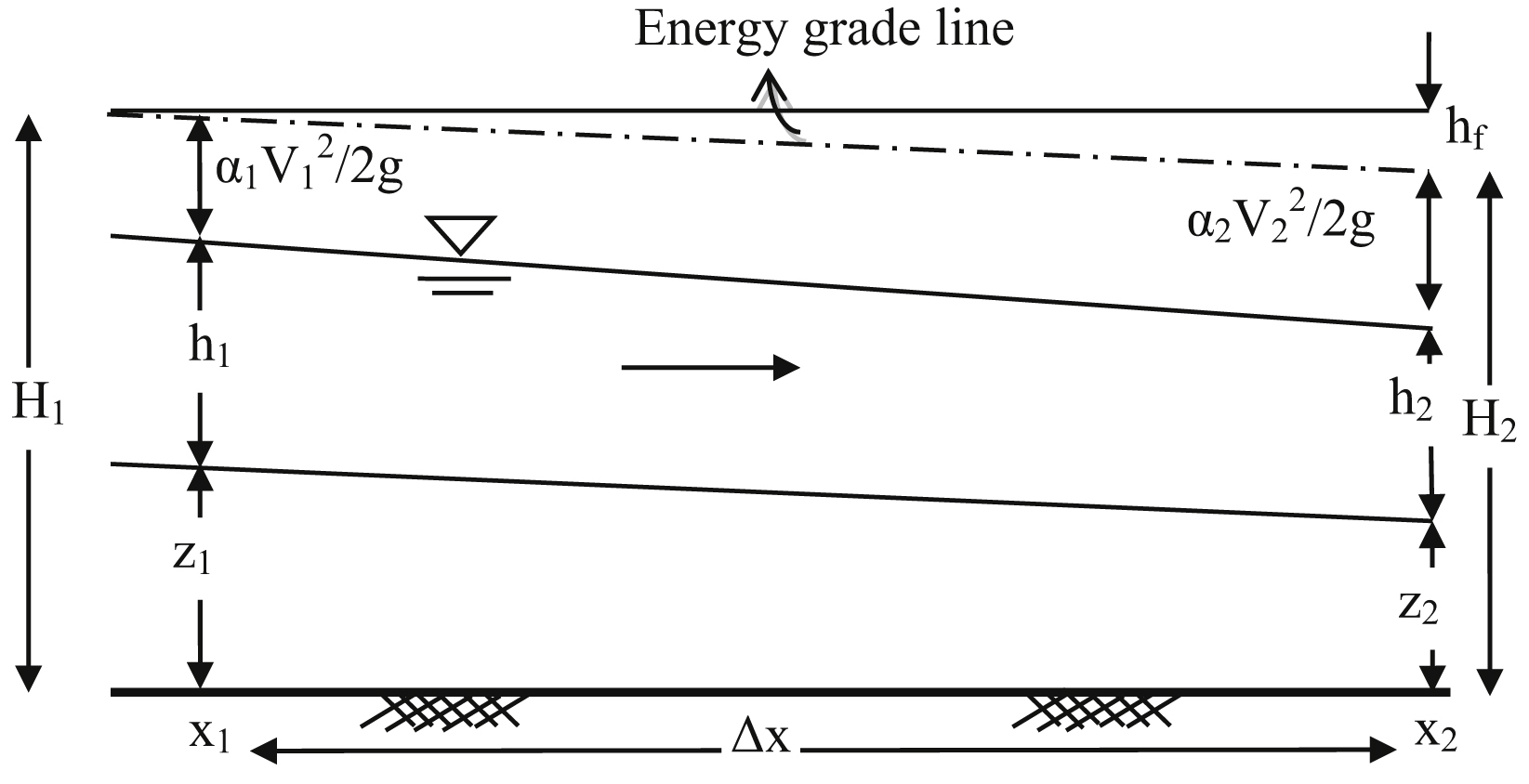
3.6.2.3. Standard Step Method

In the previous method, it is difficult to determine the flow depth at specified locations. To overcome this, a method called standard step method has been developed (Chow, 1959; Chaudhry, 2008). This method is the basis for a popular computer program known as HEC-RAS developed by Hydrologic Engineering Center, US Army Corps of Engineers.

In Fig. 3.10, the flow depth h₁ for the specified discharge Q at section 1 (i.e., at location x₁) is known and we have to determine the flow depth h₂ at location x₂ (section 2). Since h₁ and channel geometry are known, other hydraulic parameters can be determined, such as A₁, P₁, R₁, and V₁ followed by total head H₁ using the energy equation as:

$H_{1} = z_{1} + h_{1} + \frac{α_{1} V_{1}^{2}}{2 g}$ $H_{1} = z_{1} + h_{1} + \frac{α_{1} V_{1}^{2}}{2 g}$

(3.165)

According to energy equation, the total head at section 2 will be

$H_{2} = H_{1} - h_{f}$ $H_{2} = H_{1} - h_{f}$

(3.166)

The value of h_f can be determined by the average friction or energy slope as:

$h_{f} = \frac{1}{2} (S_{f 1} + S_{f 2}) \cdot (x_{2} - x_{1})$ $h_{f} = \frac{1}{2} (S_{f 1} + S_{f 2}) \cdot (x_{2} - x_{1})$

(3.167)

Figure 3.10 Computation of flow depth at distance x₂.

Substituting H₁ from Eq. (3.165) and h_f from Eq. (3.167) into Eq. (3.166),

$H_{2} = H_{1} - \frac{1}{2} (S_{f 1} + S_{f 2}) \cdot (x_{2} - x_{1})$ $H_{2} = H_{1} - \frac{1}{2} (S_{f 1} + S_{f 2}) \cdot (x_{2} - x_{1})$

(3.168)

Substituting Eq. (3.165) with subscripts and rearranging the terms results in the following form of governing equation for determining the water surface profile:

$h_{2} + \frac{α_{2} Q^{2}}{2 g A_{2}^{2}} + z_{2} + \frac{1}{2} S_{f 2} (x_{2} - x_{1}) - H_{1} + \frac{1}{2} S_{f 1} \cdot (x_{2} - x_{1}) = 0$ $h_{2} + \frac{α_{2} Q^{2}}{2 g A_{2}^{2}} + z_{2} + \frac{1}{2} S_{f 2} (x_{2} - x_{1}) - H_{1} + \frac{1}{2} S_{f 1} \cdot (x_{2} - x_{1}) = 0$

(3.169)

In Eq. (3.169), A₂ and S_f2 are functions of h₂, and other quantities are known at section 1. Hence h₂ may be determined by solving the following nonlinear algebraic equation using either a trial-and-error method or the Newton–Rapson method (Chaudhry, 2008).

$F (h_{2}) = h_{2} + \frac{α_{2} Q^{2}}{2 g A_{2}^{2}} + z_{2} + \frac{1}{2} S_{f 2} (x_{2} - x_{1}) - H_{1} + \frac{1}{2} S_{f 1} \cdot (x_{2} - x_{1}) = 0$ $F (h_{2}) = h_{2} + \frac{α_{2} Q^{2}}{2 g A_{2}^{2}} + z_{2} + \frac{1}{2} S_{f 2} (x_{2} - x_{1}) - H_{1} + \frac{1}{2} S_{f 1} \cdot (x_{2} - x_{1}) = 0$

(3.170)

For using the Newton–Rapson method, an expression

\frac{d F_{2}}{d h_{2}}

$\frac{d F_{2}}{d h_{2}}$

will be required and is derived by Chaudhry (2008) using

S_{f} = {(\frac{n Q}{A R^{2 / 3}})}^{2}

$S_{f} = {(\frac{n Q}{A R^{2 / 3}})}^{2}$

$\frac{d F_{2}}{d h_{2}} = 1 - \frac{α_{2} Q^{2} B_{2}}{g A_{2}^{3}} - (x_{2} - x_{1}) (S_{f 2} \frac{B_{2}}{A_{2}} + \frac{2}{3} \frac{S_{f 2}}{R_{2}} \frac{d R_{2}}{d h_{2}})$ $\frac{d F_{2}}{d h_{2}} = 1 - \frac{α_{2} Q^{2} B_{2}}{g A_{2}^{3}} - (x_{2} - x_{1}) (S_{f 2} \frac{B_{2}}{A_{2}} + \frac{2}{3} \frac{S_{f 2}}{R_{2}} \frac{d R_{2}}{d h_{2}})$

(3.171)

The term

\frac{d R_{2}}{d h_{2}}

$\frac{d R_{2}}{d h_{2}}$

is given by the following expression:

$\frac{d R_{2}}{d h_{2}} = \frac{B_{2}}{P_{2}} - \frac{A_{2}}{P_{2}^{2}} \frac{d P_{2}}{d h_{2}}$ $\frac{d R_{2}}{d h_{2}} = \frac{B_{2}}{P_{2}} - \frac{A_{2}}{P_{2}^{2}} \frac{d P_{2}}{d h_{2}}$

(3.172)

in which

$\begin{matrix} \frac{d P_{2}}{d h_{2}} = 2; & for rectangular channel \\ \frac{d P_{2}}{d h_{2}} = 2 \sqrt{1 + z^{2}}; & for trapezoidal channel \end{matrix}$ $\begin{matrix} \frac{d P_{2}}{d h_{2}} = 2; & for rectangular channel \\ \frac{d P_{2}}{d h_{2}} = 2 \sqrt{1 + z^{2}}; & for trapezoidal channel \end{matrix}$

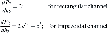(3.173)

where z is the side slope of the bank (H:V).

With an assumed value of

h_{2}^{*}

$h_{2}^{*}$

, the terms can be estimated, followed by estimating the refined value of h₂ using the following formula:

$h_{2} = h_{2}^{*} - \frac{F (h_{2}^{*})}{[d F / d h_{2}^{*}]}$ $h_{2} = h_{2}^{*} - \frac{F (h_{2}^{*})}{[d F / d h_{2}^{*}]}$

(3.174)

| h_{2} - h_{2}^{*} | < ε

$| h_{2} - h_{2}^{*} | < ε$

then

h_{2}^{*} = h_{2}

$h_{2}^{*} = h_{2}$

, otherwise the previous computation will be repeated for a new value of

h_{2}^{*}

$h_{2}^{*}$

The step-by-step procedure of computing the water surface profile using the standard step method employing the Newton–Rapson method is summarized as follows:

1. Compute the total head H₁ at section 1 from Eq. (3.165) for known values of h₁ and z₁.

2. Estimate the initial value of flow depth at section 2, i.e., h₂ using Eq. (3.150) as:

$f (x_{1}, h_{1}) = \frac{d h}{d x} = \frac{S_{0} - S_{f}}{1 - F_{r}^{2}} = \frac{S_{0} - S_{f}}{1 - \frac{T Q^{2}}{g A^{3}}}$ $f (x_{1}, h_{1}) = \frac{d h}{d x} = \frac{S_{0} - S_{f}}{1 - F_{r}^{2}} = \frac{S_{0} - S_{f}}{1 - \frac{T Q^{2}}{g A^{3}}}$

(3.175)

$h_{2}^{*} = h_{1} + f (x_{1}, h_{1}) (x_{2} - x_{1})$ $h_{2}^{*} = h_{1} + f (x_{1}, h_{1}) (x_{2} - x_{1})$

(3.176)

3. Using the estimated value of

h_{2}^{*}

$h_{2}^{*}$

, determine

B_{2}^{*}, A_{2}^{*}, P_{2}^{*}, R_{2}^{*}

$B_{2}^{*}, A_{2}^{*}, P_{2}^{*}, R_{2}^{*}$

, and

S_{f 2}^{*}

$S_{f 2}^{*}$

. The value of z₂ is either given or computed from the longitudinal bed slope and channel reach length.

4. Compute the value of F(

h_{2}^{*}

$h_{2}^{*}$

) from Eq. (3.170) using the value of

B_{2}^{*}, A_{2}^{*}, P_{2}^{*}, R_{2}^{*}

$B_{2}^{*}, A_{2}^{*}, P_{2}^{*}, R_{2}^{*}$

, and

S_{f 2}^{*}

$S_{f 2}^{*}$

5. Compute dF/dh₂ from Eq. (3.171) using

h_{2}^{*}

$h_{2}^{*}$

and the corresponding value of

B_{2}^{*}, A_{2}^{*}, P_{2}^{*}, R_{2}^{*}

$B_{2}^{*}, A_{2}^{*}, P_{2}^{*}, R_{2}^{*}$

S_{f 2}^{*}

$S_{f 2}^{*}$

, etc.

6. A better estimate for

h_{2}^{*}

$h_{2}^{*}$

is then computed using the following formula:

$h_{2} = h_{2}^{*} - \frac{F (h_{2}^{*})}{[d F / d h_{2}^{*}]}$ $h_{2} = h_{2}^{*} - \frac{F (h_{2}^{*})}{[d F / d h_{2}^{*}]}$

(3.177)

7. If

| h_{2} - h_{2}^{*} | \leq ε

$| h_{2} - h_{2}^{*} | \leq ε$

[ɛ is the specified tolerance, (say 0.001 m)], then

h_{2}^{*}

$h_{2}^{*}$

is the flow depth h₂. If the condition is not satisfied, then steps 3–7 will be repeated for new value of

h_{2}^{*}

$h_{2}^{*}$

(i.e.,

h_{2}^{*}

$h_{2}^{*}$

= h₂).

3.6.2.4. Predictor–Corrector Method

In the predictor–corrector method, we consider subcritical flow in which the direction of integration will be upstream.

Let x_n be the starting point where h_n is known for the specified discharge Q and Δx is the step length so that x_n+1 = x_n − Δx, (x_n+1 is the upstream location of x_n). At x_n with the given value of h_n and Q, the total head can be determined. Denoting

$F (h) = \frac{S_{0} - S_{f} (h)}{1 - F_{r}^{2} (h)}$ $F (h) = \frac{S_{0} - S_{f} (h)}{1 - F_{r}^{2} (h)}$

(3.178)

the flow can be computed using Euler's step scheme as:

$\frac{d h}{d x} = \frac{h_{n} - h_{n + 1}}{Δ x} = F (h_{n})$ $\frac{d h}{d x} = \frac{h_{n} - h_{n + 1}}{Δ x} = F (h_{n})$

(3.179)

$h_{n + 1} = h_{n} - F (h_{n}) \cdot Δ x$ $h_{n + 1} = h_{n} - F (h_{n}) \cdot Δ x$

(3.180)

whereas the predictor-corrector scheme will be

$h_{pred} = h_{n} - F (h_{n}) \cdot Δ x$ $h_{pred} = h_{n} - F (h_{n}) \cdot Δ x$

(3.181)

$h_{corr} = h_{n + 1} = h_{n} - 0.5 [F (h_{n}) + F (h_{pred})] \cdot Δ x$ $h_{corr} = h_{n + 1} = h_{n} - 0.5 [F (h_{n}) + F (h_{pred})] \cdot Δ x$

(3.182)

Example 3.17:

A rectangular concrete channel (n = 0.015) has a width of 7 m and longitudinal slope of 0.001 and carries a discharge of 12 m³/s. The water depth measured at the gauging location is 0.90 m. Use the direct integration method to determine the flow depth 100 and 200 m upstream of the gauging station (Table 3.10).

Solution:

Given: Channel section: rectangular; channel width, B = 7.0 m; Manning's n = 0.015, S₀ = 0.001 m/m; Q = 12 m³/s; h₀ = 0.90 m.

Example 3.18:

A rectangular concrete channel (n = 0.015) has a width of 7 m and a longitudinal slope of 0.001 and carries a discharge of 12 m³/s. The water depth measured at the gauging location is 0.90 m. Use the direct integration method to determine the flow depth of 100 and 200 m upstream of the gauging station.

Solution:

Given: Q = 12 m³/s, channel section = rectangular; bottom width, B = 7.0 m; longitudinal slope S₀ = 0.001; Manning's n = 0.015; flow depth at gauging site, h₀ = 0.90 m.

Computation: upstream direction;

x₁: downstream location;

x₂: upstream location.

Computational table is presented as a table. The columnwise description is summarized as below.

Col. (i): Assumed depth in the upstream direction of gauging station for which distance is to be computed;

Col. (ii)–(v): Hydraulic parameters corresponding to known value of flow depth either given or computed during previous step, discharge, and channel geometry;

Col. (vi): Slope of the energy grade line for computed flow parameters [Col. (ii) an (iv) along with Manning's n and Q];

Col. (vii): Specific energy using the value in Col. (i) and Col. (v);

Col. (viii)–(xiii): Flow parameters corresponding to the flow depth in the upstream direction for which distance x₂ will be determined;

Col. (xiv): Difference in specific energy between consecutive sections;

Col. (xv): Δx will be computed using

Δ x = \frac{Δ E}{S_{0} - 0.5 (S_{f 1} + S_{f 2})}

$Δ x = \frac{Δ E}{S_{0} - 0.5 (S_{f 1} + S_{f 2})}$

;

Col. (xvi): Distance of the upstream section from the gauging station is determined using: x₂ = x₁ + Δx (Table 3.11).

Table 3.10

Computation of Water Surface Profile Using the Direct Integration Method (Trial-and-Error Approach)

x	x₂ − x₁	H	$h_{2}^{}$ $h_{2}^{}$	$\bar{h}$ $\bar{h}$ (m)	$\bar{A}$ $\bar{A}$	$\bar{P}$ $\bar{P}$	$\bar{R}$ $\bar{R}$	$\bar{T}$ $\bar{T}$	$\bar{D}$ $\bar{D}$	$\bar{V}$ $\bar{V}$	${\bar{F}}_{r}$ ${\bar{F}}_{r}$	${\bar{S}}_{f}$ ${\bar{S}}_{f}$	F(x,h)	${\hat{h}}_{2}$ ${\hat{h}}_{2}$
(i)	(ii)	(iii)	(iv)	(v)	(vi)	(vii)	(viii)	(ix)	(x)	(xi)	(xii)	(xiii)	(xiv)	(xv)
0		0.9
∗100	100	0.9335	0.9335	0.91675	6.41725	8.8335	0.726467	7	0.91675	1.86996	0.623551494	0.001204763	−0.00034	0.933503
150	50	0.9431	0.9431	0.9383	6.5681	8.8766	0.739934	7	0.9383	1.827012	0.602193589	0.001122234	−0.00019	0.943089
200	50	0.9502	0.9502	0.94665	6.62655	8.8933	0.745117	7	0.94665	1.810897	0.594243642	0.00109231	−0.00014	0.950235
300	100	0.9599	0.9598	0.955	6.685	8.91	0.750281	7	0.955	1.795064	0.586467088	0.001063454	−0.00010	0.959872
400	100	0.9656	0.9655	0.9627	6.7389	8.9254	0.755025	7	0.9627	1.780706	0.579445033	0.001037751	−0.00006	0.965583
523	123	0.9696	0.9696	0.9676	6.7732	8.9352	0.758036	7	0.9676	1.771688	0.57504908	0.001021831	−0.00003	0.969612

Example 3.19:

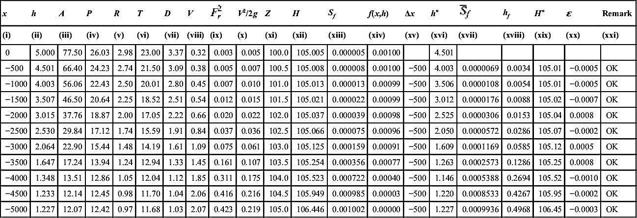
A trapezoidal channel with a side slope of 1.5 (H:V) having a bottom width of 8.0 m and a longitudinal slope of 0.001 is carrying a discharge of 25 m³/s. A control structure is built at the downstream end, which raises the water depth at the downstream end to 5.0 m, where the channel bed level is 100 m. Compute the water surface profile using the direct step method. Assume Manning's n as 0.015.

Solution:

Given section = trapezoidal; bottom width, B = 8.0 m; side slope, z = 1.5; discharge, Q = 25 m³/s; Manning's n = 0.015; water depth at the control structure, h₀ = 5.0 m; and channel bed elevation at control structure = 100.0 m.

Computational method: direct step.

Computation direction: upstream (Tables 3.12 and 3.13).

The bed elevation is determined: the bed elevation at the control structure, distance upstream, and longitudinal slope of the channel. The elevation of the water surface is determined by adding the channel bed level and the bed level. The water surface profile so obtained is depicted in Figs. 3.11 and 3.12.

Example 3.20:

Solution:

Given section = trapezoidal; bottom width, B = 8.0 m; side slope, z = 1.5; discharge, Q = 25 m³/s; Manning's n = 0.015; water depth at the control structure, h₀ = 5.0 m; channel bed elevation at control structure = 100.0 m. Computational method will be the standard step with a trial-and-error method (Table 3.14).

Plot of the water surface profile is depicted in Fig. 3.13.

Example 3.21:

Solution:

Given: Section = trapezoidal; bottom width, B = 8.0 m; side slope, z = 1.5; discharge, Q = 25 m³/s; Manning's n = 0.015; water depth at the control structure, h₀ = 5.0 m; channel bed elevation at control structure = 100.0 m.

Table 3.11

Computation of Water Surface Profile Using Direct Step Method

h₁	A₁	P₁	R₁	V₁	S_f1	E₁	A₂	P₂	R₂	V₂	S_f2	E₂	ΔE	Δx	x₂
(i)	(ii)	(iii)	(iv)	(v)	(vi)	(vii)	(viii)	(ix)	(x)	(xi)	(xii)	(xiii)	(xiv)	(xv)	(xvi)
0.90	6.30	8.80	0.7159	1.9048	0.0012747	1.0849									0
0.91	6.37	8.82	0.7222	1.8838	0.0012323	1.0909	6.37	8.82	0.7222	1.8838	0.0012323	1.0909	0.0060	−23.5055	−23.5055
0.92	6.44	8.84	0.7285	1.8634	0.0011918	1.0970	6.44	8.84	0.7285	1.8634	0.0011918	1.0970	0.0061	−28.7163	−52.2218
0.93	6.51	8.86	0.7348	1.8433	0.0011531	1.1032	6.51	8.86	0.7348	1.8433	0.0011531	1.1032	0.0062	−36.0389	−88.2606
0.94	6.58	8.88	0.7410	1.8237	0.0011161	1.1095	6.58	8.88	0.7410	1.8237	0.0011161	1.1095	0.0063	−47.075	−135.336
0.95	6.65	8.90	0.7472	1.8045	0.0010806	1.1160	6.65	8.90	0.7472	1.8045	0.0010806	1.1160	0.0065	−65.5956	−200.931
0.96	6.72	8.92	0.7534	1.7857	0.0010467	1.1225	6.72	8.92	0.7534	1.7857	0.0010467	1.1225	0.0066	−103.09	−304.021
0.97	6.79	8.94	0.7595	1.7673	0.0010142	1.1292	6.79	8.94	0.7595	1.7673	0.0010142	1.1292	0.0067	−219.207	−523.228

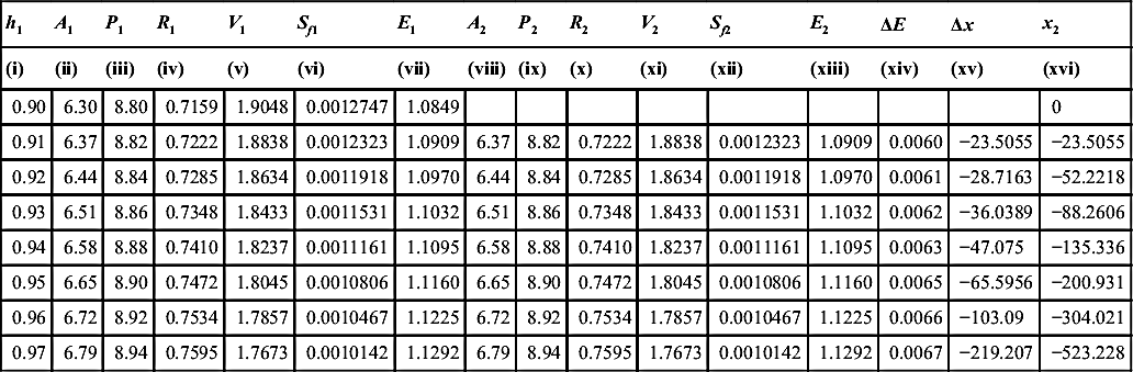
Table 3.12

Computation of Water Surface Profile Using the Direct Step Method When the Control Structure Is Provided Downstream

h₁	A₁	P₁	R₁	V₁	S_f1	E₁	A₂	P₂	R₂	V₂	S_f2	E₂	ΔE	Δx	x₂
(i)	(ii)	(iii)	(iv)	(v)	(vi)	(vii)	(viii)	(ix)	(x)	(xi)	(xii)	(xiii)	(xiv)	(xv)	(xvi)
5.00	77.500	26.028	2.9776	0.3226	0.0000055	5.005									0
4.50	66.375	24.225	2.7399	0.3766	0.0000083	4.507	66.375	24.225	2.7399	0.3766	0.000008	4.50723	−0.4981	−501.531	−501.53
4.00	56.000	22.422	2.4975	0.4464	0.0000132	4.010	56.000	22.422	2.4975	0.4464	0.000013	4.01016	−0.4971	−502.489	−1004.02
3.50	46.375	20.619	2.2491	0.5391	0.0000222	3.515	46.375	20.619	2.2491	0.5391	0.000022	3.51481	−0.4953	−504.277	−1508.30
3.25	41.844	19.718	2.1221	0.5975	0.0000295	3.268	41.844	19.718	2.1221	0.5975	0.000029	3.26819	−0.2466	−253.155	−1761.45
3.00	37.500	18.817	1.9929	0.6667	0.0000399	3.023	37.500	18.817	1.9929	0.6667	0.000040	3.02265	−0.2455	−254.357	−2015.81
2.75	33.344	17.915	1.8612	0.7498	0.0000552	2.779	33.344	17.915	1.8612	0.7498	0.000055	2.77865	−0.2440	−256.184	−2271.99
2.50	29.375	17.014	1.7265	0.8511	0.0000787	2.537	29.375	17.014	1.7265	0.8511	0.000079	2.53692	−0.2417	−259.084	−2531.08
2.25	25.594	16.112	1.5884	0.9768	0.0001158	2.299	25.594	16.112	1.5884	0.9768	0.000116	2.29863	−0.2383	−263.957	−2795.03
2.00	22.000	15.211	1.4463	1.1364	0.0001776	2.066	22.000	15.211	1.4463	1.1364	0.000178	2.06582	−0.2328	−272.85	−3067.88
1.80	19.260	14.490	1.3292	1.2980	0.0002594	1.886	19.260	14.490	1.3292	1.2980	0.000259	1.88588	−0.1799	−230.255	−3298.14
1.60	16.640	13.769	1.2085	1.5024	0.0003945	1.715	16.640	13.769	1.2085	1.5024	0.000395	1.71505	−0.1708	−253.816	−3551.96
1.40	14.140	13.048	1.0837	1.7680	0.0006318	1.559	14.140	13.048	1.0837	1.7680	0.000632	1.55932	−0.1557	−319.881	−3871.84
1.30	12.935	12.687	1.0195	1.9327	0.0008191	1.490	12.935	12.687	1.0195	1.9327	0.000819	1.49039	−0.0689	−251.089	−4122.92
1.20							11.760	12.327	0.9540	2.1259	0.001083	1.43034	−0.0601	−1222.65	−5345.57

Table 3.13

Computation of Water Surface Profile

h	5.0	4.5	4.0	3.5	3.3	3.0	2.8	2.5	2.3	2.0	1.8	1.6	1.4	1.3	1.2
EL-bed	100.000	100.502	101.004	101.508	101.761	102.016	102.272	102.531	102.795	103.068	103.298	103.552	103.872	104.123	105.346
EL-WS (m)	105.000	105.002	105.004	105.008	105.011	105.016	105.022	105.031	105.045	105.068	105.098	105.152	105.272	105.423	106.546

Figure 3.11 Flow depth upstream of the control structure.

Figure 3.12 Water surface profile upstream of the control structure.

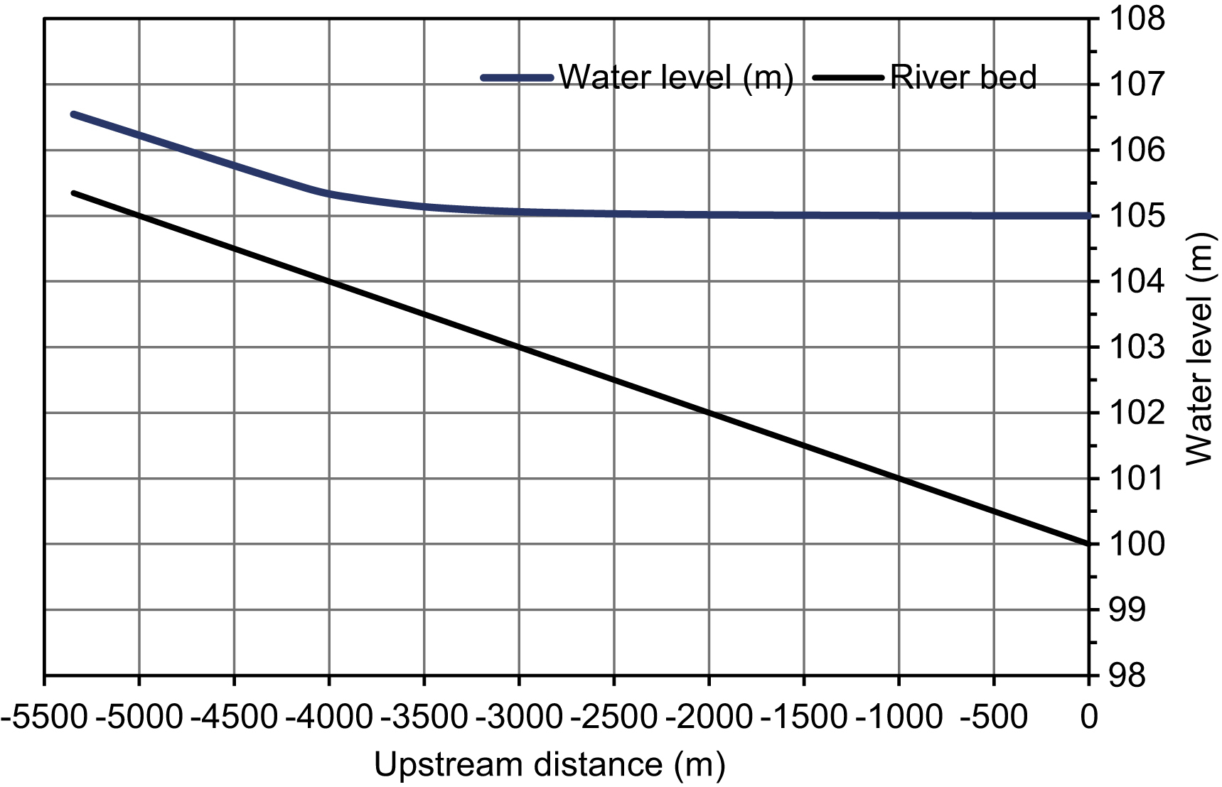
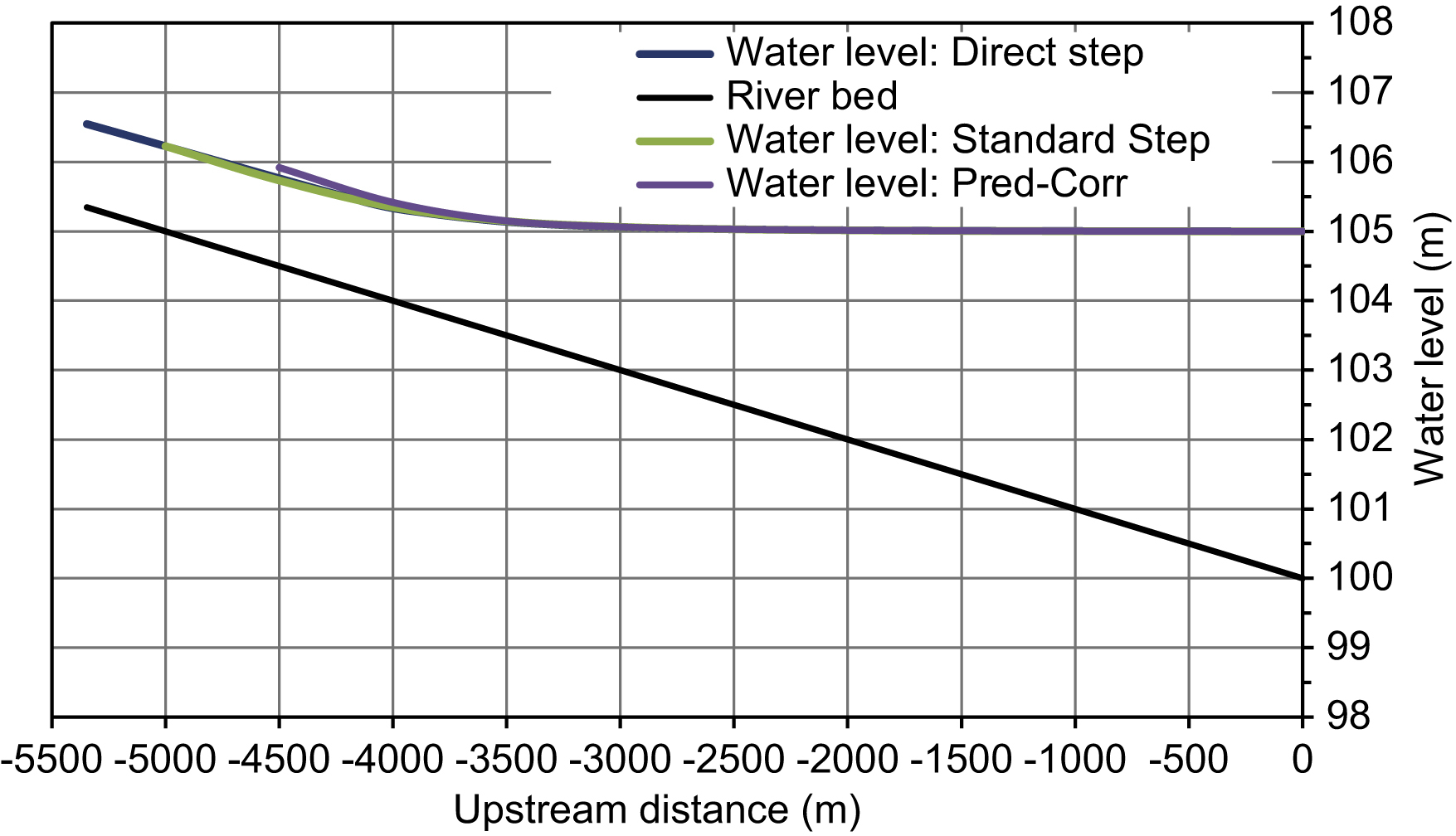
Table 3.14

Computation of Water Surface Profile Using Standard the Step Method With a Trial-and-Error Approach

x	h	A	P	R	T	D	V	$F_{r}^{2}$ $F_{r}^{2}$	V²/2g	Z	H	S_f	f(x,h)	Δx	h^∗	${\bar{S}}_{f}$ ${\bar{S}}_{f}$	h_f	H^∗	ɛ	Remark
(i)	(ii)	(iii)	(iv)	(v)	(vi)	(vii)	(viii)	(ix)	(x)	(xi)	(xii)	(xiii)	(xiv)	(xv)	(xvi)	(xvii)	(xviii)	(xix)	(xx)	(xxi)
0	5.000	77.50	26.03	2.98	23.00	3.37	0.32	0.003	0.005	100.0	105.005	0.000005	0.00100		4.501
−500	4.501	66.40	24.23	2.74	21.50	3.09	0.38	0.005	0.007	100.5	105.008	0.000008	0.00100	−500	4.003	0.0000069	0.0034	105.01	−0.0005	OK
−1000	4.003	56.06	22.43	2.50	20.01	2.80	0.45	0.007	0.010	101.0	105.013	0.000013	0.00099	−500	3.506	0.0000108	0.0054	105.01	−0.0005	OK
−1500	3.507	46.50	20.64	2.25	18.52	2.51	0.54	0.012	0.015	101.5	105.021	0.000022	0.00099	−500	3.012	0.0000176	0.0088	105.02	−0.0007	OK
−2000	3.015	37.76	18.87	2.00	17.05	2.22	0.66	0.020	0.022	102.0	105.037	0.000039	0.00098	−500	2.525	0.0000306	0.0153	105.04	0.0008	OK
−2500	2.530	29.84	17.12	1.74	15.59	1.91	0.84	0.037	0.036	102.5	105.066	0.000075	0.00096	−500	2.050	0.0000572	0.0286	105.07	−0.0002	OK
−3000	2.064	22.90	15.44	1.48	14.19	1.61	1.09	0.075	0.061	103.0	105.125	0.000159	0.00091	−500	1.609	0.0001169	0.0585	105.12	0.0005	OK
−3500	1.647	17.24	13.94	1.24	12.94	1.33	1.45	0.161	0.107	103.5	105.254	0.000356	0.00077	−500	1.263	0.0002573	0.1286	105.25	0.0008	OK
−4000	1.348	13.51	12.86	1.05	12.04	1.12	1.85	0.311	0.175	104.0	105.523	0.000722	0.00040	−500	1.146	0.0005388	0.2694	105.52	−0.0010	OK
−4500	1.233	12.14	12.45	0.98	11.70	1.04	2.06	0.416	0.216	104.5	105.949	0.000985	0.00003	−500	1.220	0.0008533	0.4267	105.95	−0.0002	OK
−5000	1.227	12.07	12.42	0.97	11.68	1.03	2.07	0.423	0.219	105.0	106.446	0.001002	0.00000	−500	1.227	0.0009936	0.4968	106.45	−0.0003	OK

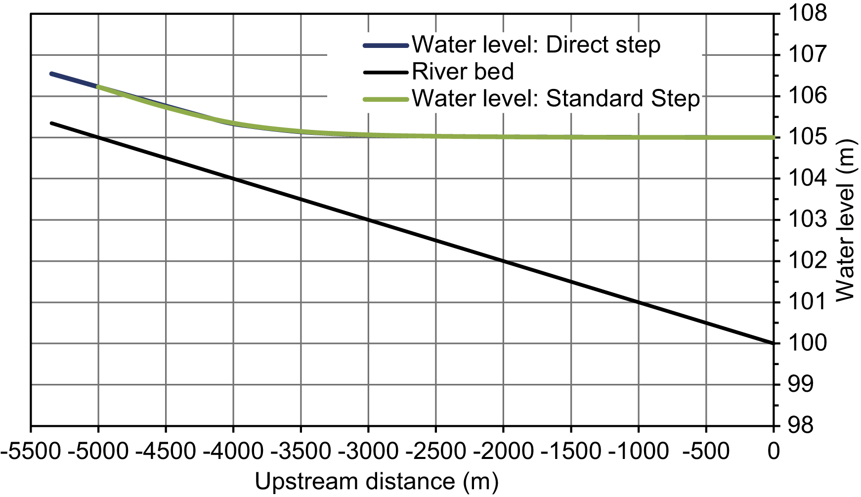
Figure 3.13 Water surface profile estimated using the standard step method and its comparison with the result of direct step method.

Computational method: Predictor–corrector method (Table 3.15).

Computation of water surface profile is given as follows, and depicted in Fig. 3.14.

x	0	−500	−1000	−1500	−2000	−2500	−3000	−3500	−4000	−4500
Bed level, z	100.0	100.5	101.0	101.5	102.0	102.5	103.0	103.5	104.0	104.5
Water level	105	105.0015	105.0039	105.008	105.0155	105.0302	105.0632	105.1503	105.4173	105.9188

Table 3.15

Computation of Water Surface Profile Using the Predictor–Corrector Method for the First Iteration

x₁	x₂	Δx	h₁	A₁	P₁	R₁	T₁	D₁	V₁	$F_{r 1}^{2}$ $F_{r 1}^{2}$	S_f1	F(x,h₁)	h_{2, pred}	A₂	P₂	R₂	T₂	D₂	V₂	$F_{r 2}^{2}$ $F_{r 2}^{2}$	S_f2	F(x,h₂)	h_{2, corr}
0	−500	500	5.000	77.50	26.03	2.98	23.00	3.37	0.32	0.0031	5.47E−06	0.000998	4.501	66.40	24.23	2.74	21.50	3.09	0.38	0.0047	8.32E−06	0.000996	4.501
−500	−1000	500	4.501	66.41	24.23	2.74	21.50	3.09	0.38	0.0047	8.31E−06	0.000996	4.003	56.07	22.43	2.50	20.01	2.80	0.45	0.0072	1.32E−05	0.000994	4.004
−1000	−1500	500	4.004	56.08	22.44	2.50	20.01	2.80	0.45	0.0072	1.32E−05	0.000994	3.507	46.50	20.64	2.25	18.52	2.51	0.54	0.0117	2.20E−05	0.00099	3.508
−1500	−2000	500	3.508	46.52	20.65	2.25	18.52	2.51	0.54	0.0117	2.20E−05	0.000990	3.013	37.72	18.86	2.00	17.04	2.21	0.66	0.0202	3.92E−05	0.000981	3.015
−2000	−2500	500	3.015	37.76	18.87	2.00	17.05	2.22	0.66	0.0202	3.91E−05	0.000981	2.525	29.77	17.10	1.74	15.58	1.91	0.84	0.0376	7.58E−05	0.00096	2.530
−2500	−3000	500	2.530	29.84	17.12	1.74	15.59	1.91	0.84	0.0374	7.53E−05	0.000961	2.050	22.70	15.39	1.48	14.15	1.60	1.10	0.0770	1.62E−04	0.000907	2.063
−3000	−3500	500	2.063	22.89	15.44	1.48	14.19	1.61	1.09	0.0754	1.59E−04	0.000910	1.608	16.75	13.80	1.21	12.82	1.31	1.49	0.1740	3.87E−04	0.000742	1.650
−3500	−4000	500	1.650	17.29	13.95	1.24	12.95	1.33	1.45	0.1597	3.53E−04	0.000769	1.266	12.53	12.56	1.00	11.80	1.06	2.00	0.3823	8.99E−04	0.000163	1.417
−4000	−4500	500	1.417	14.35	13.11	1.09	12.25	1.17	1.74	0.2641	6.05E−04	0.000536	1.149	11.17	12.14	0.92	11.45	0.98	2.24	0.5229	1.26E−03	−0.00054	1.419
−4500	−5000	500	1.419	14.37	13.12	1.10	12.26	1.17	1.74	0.2632	6.03E−04	0.000539	1.149	11.18	12.14	0.92	11.45	0.98	2.24	0.5225	1.26E−03	−0.00054	1.419