4.3. Hydrologic Equation and Water Balance

Search in book...
Toggle Font Controls
Create new playlist

Name your new playlist

Playlist description (optional)
Sign In

Email address

Password

Forgot Password?

or

Continue with Facebook

Continue with Google
Sign Up

Full Name

Email address

Confirm Email Address

Password

or

Continue with Facebook

Continue with Google

4.3. Hydrologic Equation and Water Balance

Hydrologic equation is based on the continuity equation, and can also be referred to as the water-balance equation. It is an accounting procedure for all inflows, outflows, and storages involved in the hydrologic system having a firm boundary for a specified duration or period (Fig. 4.3).

Considering the above catchment description (Fig. 4.3) and lower boundary up to the end of confined aquifer, the total inflows, total outflows, and storages involved in the catchment are defined as follows:

$Inflows, I = P + Im + G_{i} + G_{w}$ $Inflows, I = P + Im + G_{i} + G_{w}$

(4.14)

$Outflows, O = R + G_{o} + E T + E + E x$ $Outflows, O = R + G_{o} + E T + E + E x$

(4.15)

$Storages, S = S_{s} + S_{m} + S_{g}$ $Storages, S = S_{s} + S_{m} + S_{g}$

(4.16)

Note: For soil moisture storage S_m infiltration will be the input; similarly, for groundwater storage S_g, percolation will be the input.

The hydrologic equation can be expressed as (Eq. 4.17):

$I - O = \frac{Δ S}{Δ t}$ $I - O = \frac{Δ S}{Δ t}$

(4.17)

where I is the inflow (L³/T), O is the outflow (L³/T), ΔS/Δt is the change in storage in Δt period, S is the storage (L³), and t is the time interval for water balance (T). The time period may be weekly, quarterly, monthly, seasonal, or annual. For annual water balance, the hydrologic year should be considered. Eq. (4.17) may also be expressed in volumetric term when Δt is fixed, and can be presented as follows (Eq. 4.18):

$I_{Δ t} - O_{Δ t} = Δ S$ $I_{Δ t} - O_{Δ t} = Δ S$

(4.18)

In Eq. (4.18) I_Δt and O_Δt are in volumetric unit like m³ or million cubic meters (MCM), ha m, etc. These can also be expressed in depth units like mm, cm, m, etc.

Figure 4.3 Sectional view of catchment. Notation: E, evaporation; ET, evapotranspiration; Ex, exported water to other basin; F, infiltration; G_i, groundwater inflow from other basin; G_o, groundwater outflow to the other basin; G_w, groundwater withdrawal to the catchment; Im, interbasin water transfer (imported water); P, precipitation; Pr, percolation; R, runoff; S_g, groundwater storage; S_m, soil moisture storage; S_s, surface water storage; WT, water table.

Overall water balance of the catchment:

Substitution of Eqs. (4.14)–(4.16) into Eq. (4.18) results in the overall water-balance equation of the catchment's hydrologic system:

$\begin{matrix} {(P + Im + G_{i} + G_{w})}_{Δ t} \\ - {(R + E + E T + G_{o} + E x)}_{Δ t} = Δ (S_{s} + S_{m} + S_{g}) \end{matrix}$ $\begin{matrix} {(P + Im + G_{i} + G_{w})}_{Δ t} \\ - {(R + E + E T + G_{o} + E x)}_{Δ t} = Δ (S_{s} + S_{m} + S_{g}) \end{matrix}$

(4.19)

Water balance (lower boundary is catchment surface):

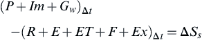$\begin{matrix} {(P + Im + G_{w})}_{Δ t} \\ - {(R + E + E T + F + E x)}_{Δ t} = Δ S_{s} \end{matrix}$ $\begin{matrix} {(P + Im + G_{w})}_{Δ t} \\ - {(R + E + E T + F + E x)}_{Δ t} = Δ S_{s} \end{matrix}$

(4.20)

Water balance (lower boundary is water table):

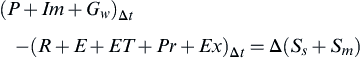$\begin{matrix} {(P + Im + G_{w})}_{Δ t} \\ - {(R + E + E T + \Pr + E x)}_{Δ t} = Δ (S_{s} + S_{m}) \end{matrix}$ $\begin{matrix} {(P + Im + G_{w})}_{Δ t} \\ - {(R + E + E T + \Pr + E x)}_{Δ t} = Δ (S_{s} + S_{m}) \end{matrix}$

(4.21)

Water balance for saturated zone (lower boundary is the first clay surface):

${(\Pr + G_{i})}_{Δ t} - {(E T + P r_{deep} + G_{w} + G_{o})}_{Δ t} = Δ S_{g}$ ${(\Pr + G_{i})}_{Δ t} - {(E T + P r_{deep} + G_{w} + G_{o})}_{Δ t} = Δ S_{g}$

(4.22)

where Pr_deep is the deep percolation.

Soil–water balance for unsaturated zone (lower boundary is water table):

$F_{Δ t} - {(E T + \Pr)}_{Δ t} = Δ S_{m}$ $F_{Δ t} - {(E T + \Pr)}_{Δ t} = Δ S_{m}$

(4.23)

4.3.1. Period of Water-Balance Exercise

For water budgeting exercise, period of analysis plays an important role in deciding the initial conditions. The period may be considered either longer or shorter, depending upon the purpose and objective of water budgeting.

Longer period may be: (1) calendar year, (2) hydrologic year, and (3) crop seasons.

Shorter period may be: (1) monthly, (2) fortnightly, (3) 10-days, (4) weekly, and (5) daily.

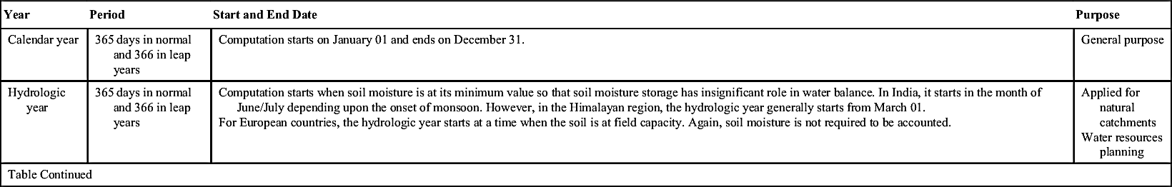
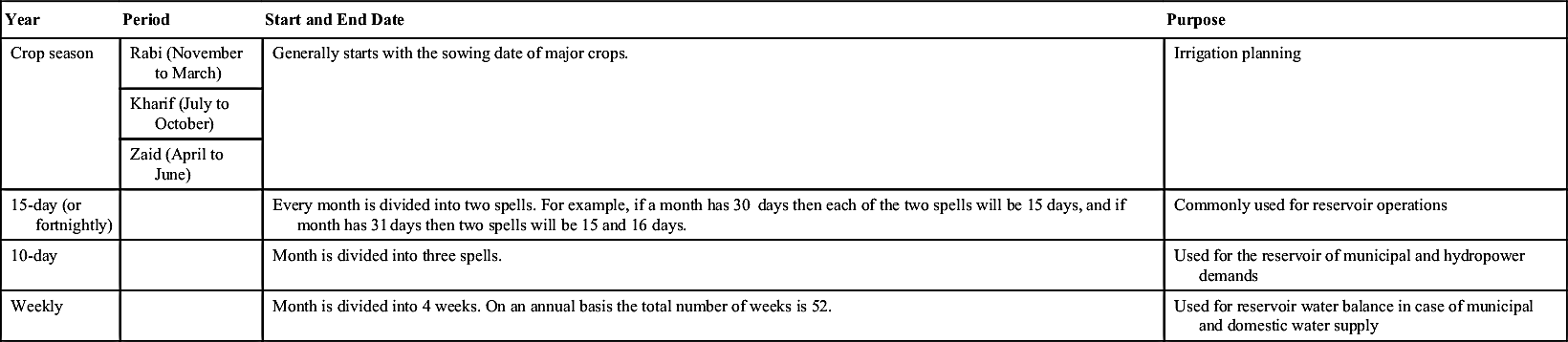
In general, the water-balance period is not considered less than a week. Table 4.5 presents guidelines for fixing the water budgeting period.

Table 4.5

Period Used in the Water-Balance Calculations

Year	Period	Start and End Date	Purpose
Calendar year	365 days in normal and 366 in leap years	Computation starts on January 01 and ends on December 31.	General purpose
Hydrologic year	365 days in normal and 366 in leap years	Computation starts when soil moisture is at its minimum value so that soil moisture storage has insignificant role in water balance. In India, it starts in the month of June/July depending upon the onset of monsoon. However, in the Himalayan region, the hydrologic year generally starts from March 01. For European countries, the hydrologic year starts at a time when the soil is at field capacity. Again, soil moisture is not required to be accounted.	Applied for natural catchments Water resources planning
Table Continued

Year	Period	Start and End Date	Purpose
Crop season	Rabi (November to March)	Generally starts with the sowing date of major crops.	Irrigation planning
	Kharif (July to October)
	Zaid (April to June)
15-day (or fortnightly)		Every month is divided into two spells. For example, if a month has 30 days then each of the two spells will be 15 days, and if month has 31 days then two spells will be 15 and 16 days.	Commonly used for reservoir operations
10-day		Month is divided into three spells.	Used for the reservoir of municipal and hydropower demands
Weekly		Month is divided into 4 weeks. On an annual basis the total number of weeks is 52.	Used for reservoir water balance in case of municipal and domestic water supply

4.3.2. Purpose of Water Balance

The water-balance exercise gives an idea of water resources availability and its use in various sectors. Other than this, water balance can be used for:

1. estimation of unknown variables for which monitoring is difficult, as for example, evapotranspiration;

2. estimation of utilization factor defined as follows:

$Factor of Utilization = \frac{Storage + Outflow}{Inflow} \times 100 %$ $Factor of Utilization = \frac{Storage + Outflow}{Inflow} \times 100 %$

(4.24)

3. water utilization exercise and estimation of surplus and deficit basin;

4. water resources planning; and

5. prefeasibility studies of interlinking projects.

Example 4.3:

During a 30 days period, the following data were observed for a single purpose reservoir (i.e., only for power generation):

Reservoir area = 500 ha

Rainfall contribution = 146 mm

Monthly evaporation = 54 mm

Other losses = 30 m³/day

Average river inflow = 110 m³/s

Power channel withdrawal = 120 m³/s

Estimate the drawdown in the reservoir considering the reservoir to be prismatic with vertical walls. Also, determine the daily drawdown curve during reservoir operation, assuming daily mean rainfall and evaporation, and initial pond level in the reservoir as 20 m.

Solution:

The monthly water balance in volumetric terms (m³) for the reservoir can be given as follows:

$Inflow - Outflow = Change in Pondage$ $Inflow - Outflow = Change in Pondage$

\bar{I} Δ t + (P - E) A_{r e s} - L Δ t - \bar{Q} Δ t = Δ S

$\bar{I} Δ t + (P - E) A_{r e s} - L Δ t - \bar{Q} Δ t = Δ S$

Terms appearing in the above equation can be worked out as follows:

$\bar{I} Δ t = (110 \times 3600 \times 24 \times 30) / 10^{6} = 285.12 MCM$ $\bar{I} Δ t = (110 \times 3600 \times 24 \times 30) / 10^{6} = 285.12 MCM$

$(P - E) A_{r e s} = [(146 - 54) / 1000] \times (500 \times 10^{4}) = 460,000 m^{3} = 0.46 MCM$ $(P - E) A_{r e s} = [(146 - 54) / 1000] \times (500 \times 10^{4}) = 460,000 m^{3} = 0.46 MCM$

$L Δ t = 30 \times 30 = 900 m^{3} = 0.0009 MCM$ $L Δ t = 30 \times 30 = 900 m^{3} = 0.0009 MCM$

$\bar{Q} Δ t = (120 \times 3600 \times 24 \times 30) / 10^{6} = 311.04 MCM$ $\bar{Q} Δ t = (120 \times 3600 \times 24 \times 30) / 10^{6} = 311.04 MCM$

Therefore the change in storage or pondage during 30 days will be:

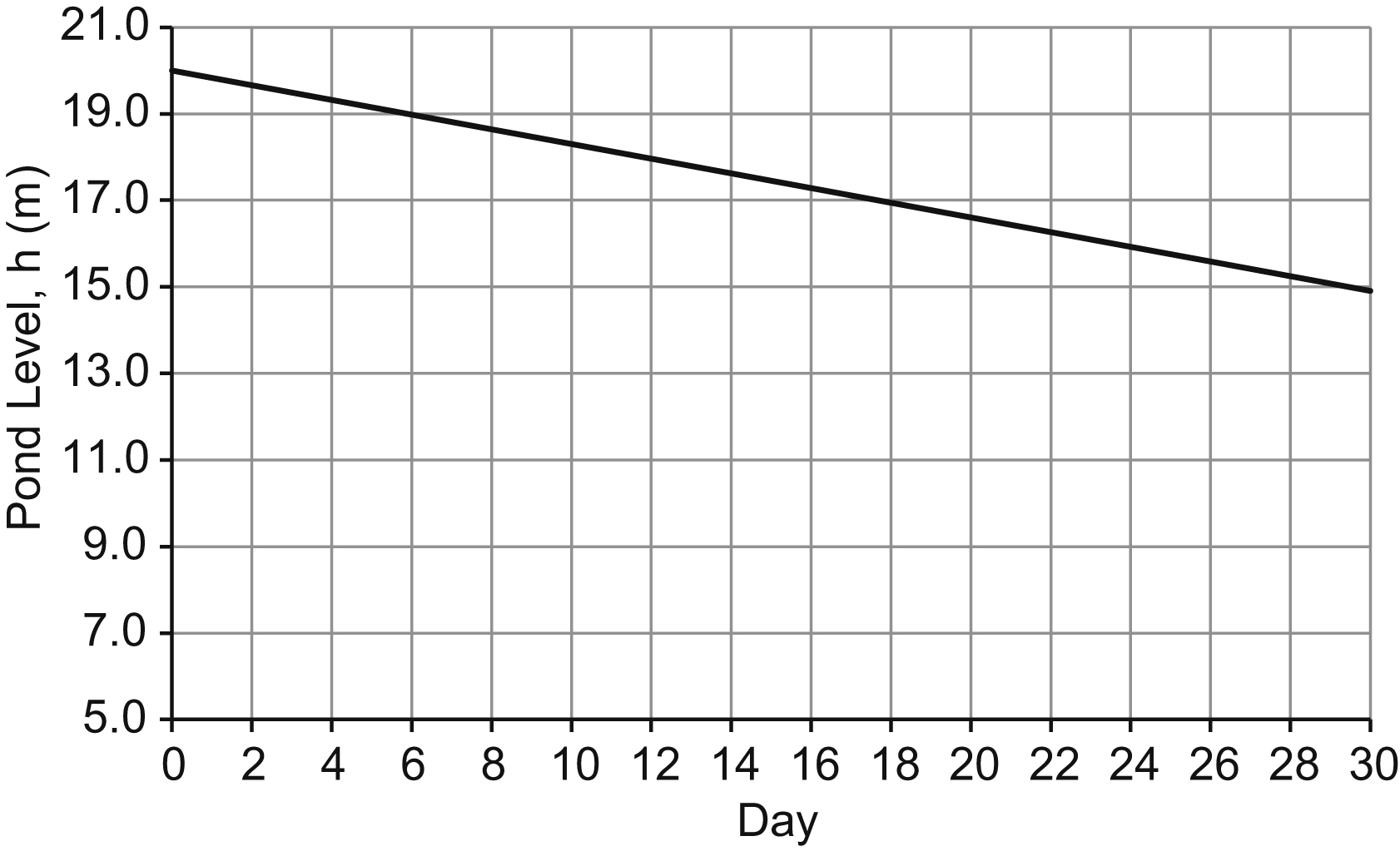
$Δ S = 285.12 + 0.460 - 0.0009 - 311.04 = - 25.46 MCM$ $Δ S = 285.12 + 0.460 - 0.0009 - 311.04 = - 25.46 MCM$

The total drawdown during the month, Δh, can be estimated using the following formula:

$Δ h = \frac{Δ S}{A_{r e s}} = \frac{25.46 \times 10^{6}}{500 \times 10^{4}} = 5.092 m$ $Δ h = \frac{Δ S}{A_{r e s}} = \frac{25.46 \times 10^{6}}{500 \times 10^{4}} = 5.092 m$

where h is the pond level (m).

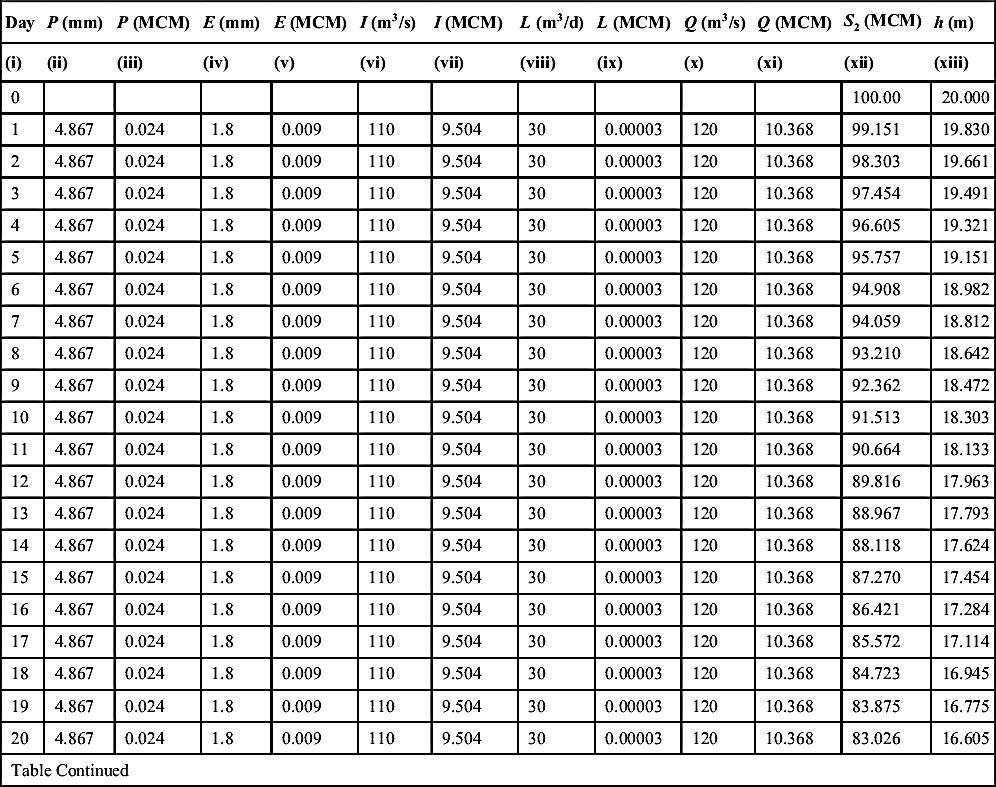
Analysis of daily reservoir water balance and drawdown is presented in Table 4.6.

Column-wise computation steps are:

(iii) = [(ii)/1000] × (A_res × 10,000)/1,000,000;

(v) = [(iv)/1000] × (A_res × 10,000)/1,000,000;

(vii) = (vi) × 3600 × 24/1,000,000;

(ix) = (viii)/1,000,000;

(xi) = (x) × 3600 × 24/1,000,000;

(xii)_t = (xii)_t−1 + (iii) + (vii) − (v) − (ix) − (xi)

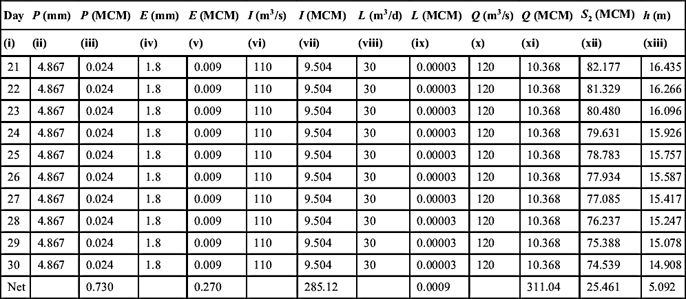
The total drawdown level in the reservoir = 20.000 − 14.908 = 5.092 m.

The drawdown curve during the operation is shown in Fig. 4.4.

Example 4.4:

Use the following data:

Reservoir area = 240 ha

Contributing rainfall = 2540 mm/year

Table 4.6

Estimation of Daily Drawdown of the Reservoir

Day	P (mm)	P (MCM)	E (mm)	E (MCM)	I (m³/s)	I (MCM)	L (m³/d)	L (MCM)	Q (m³/s)	Q (MCM)	S₂ (MCM)	h (m)
(i)	(ii)	(iii)	(iv)	(v)	(vi)	(vii)	(viii)	(ix)	(x)	(xi)	(xii)	(xiii)
0											100.00	20.000
1	4.867	0.024	1.8	0.009	110	9.504	30	0.00003	120	10.368	99.151	19.830
2	4.867	0.024	1.8	0.009	110	9.504	30	0.00003	120	10.368	98.303	19.661
3	4.867	0.024	1.8	0.009	110	9.504	30	0.00003	120	10.368	97.454	19.491
4	4.867	0.024	1.8	0.009	110	9.504	30	0.00003	120	10.368	96.605	19.321
5	4.867	0.024	1.8	0.009	110	9.504	30	0.00003	120	10.368	95.757	19.151
6	4.867	0.024	1.8	0.009	110	9.504	30	0.00003	120	10.368	94.908	18.982
7	4.867	0.024	1.8	0.009	110	9.504	30	0.00003	120	10.368	94.059	18.812
8	4.867	0.024	1.8	0.009	110	9.504	30	0.00003	120	10.368	93.210	18.642
9	4.867	0.024	1.8	0.009	110	9.504	30	0.00003	120	10.368	92.362	18.472
10	4.867	0.024	1.8	0.009	110	9.504	30	0.00003	120	10.368	91.513	18.303
11	4.867	0.024	1.8	0.009	110	9.504	30	0.00003	120	10.368	90.664	18.133
12	4.867	0.024	1.8	0.009	110	9.504	30	0.00003	120	10.368	89.816	17.963
13	4.867	0.024	1.8	0.009	110	9.504	30	0.00003	120	10.368	88.967	17.793
14	4.867	0.024	1.8	0.009	110	9.504	30	0.00003	120	10.368	88.118	17.624
15	4.867	0.024	1.8	0.009	110	9.504	30	0.00003	120	10.368	87.270	17.454
16	4.867	0.024	1.8	0.009	110	9.504	30	0.00003	120	10.368	86.421	17.284
17	4.867	0.024	1.8	0.009	110	9.504	30	0.00003	120	10.368	85.572	17.114
18	4.867	0.024	1.8	0.009	110	9.504	30	0.00003	120	10.368	84.723	16.945
19	4.867	0.024	1.8	0.009	110	9.504	30	0.00003	120	10.368	83.875	16.775
20	4.867	0.024	1.8	0.009	110	9.504	30	0.00003	120	10.368	83.026	16.605
Table Continued

Day	P (mm)	P (MCM)	E (mm)	E (MCM)	I (m³/s)	I (MCM)	L (m³/d)	L (MCM)	Q (m³/s)	Q (MCM)	S₂ (MCM)	h (m)
(i)	(ii)	(iii)	(iv)	(v)	(vi)	(vii)	(viii)	(ix)	(x)	(xi)	(xii)	(xiii)
21	4.867	0.024	1.8	0.009	110	9.504	30	0.00003	120	10.368	82.177	16.435
22	4.867	0.024	1.8	0.009	110	9.504	30	0.00003	120	10.368	81.329	16.266
23	4.867	0.024	1.8	0.009	110	9.504	30	0.00003	120	10.368	80.480	16.096
24	4.867	0.024	1.8	0.009	110	9.504	30	0.00003	120	10.368	79.631	15.926
25	4.867	0.024	1.8	0.009	110	9.504	30	0.00003	120	10.368	78.783	15.757
26	4.867	0.024	1.8	0.009	110	9.504	30	0.00003	120	10.368	77.934	15.587
27	4.867	0.024	1.8	0.009	110	9.504	30	0.00003	120	10.368	77.085	15.417
28	4.867	0.024	1.8	0.009	110	9.504	30	0.00003	120	10.368	76.237	15.247
29	4.867	0.024	1.8	0.009	110	9.504	30	0.00003	120	10.368	75.388	15.078
30	4.867	0.024	1.8	0.009	110	9.504	30	0.00003	120	10.368	74.539	14.908
Net		0.730		0.270		285.12		0.0009		311.04	25.461	5.092

Figure 4.4 Drawdown curve for the reservoir during 1 month of operation.

Mean annual inflow = 142 lps

Mean annual outflows = 125 lps

Increase in storage = 3.08 MCM

To compute the evaporation loss in MCM and mm during a period of 365 days.

Solution:

The hydrologic budget equation for this problem can be given as follows:

$P \cdot A_{r e s} - E \cdot A_{r e s} + \bar{I} Δ t - \bar{O} Δ t = Δ S$ $P \cdot A_{r e s} - E \cdot A_{r e s} + \bar{I} Δ t - \bar{O} Δ t = Δ S$

where

P \cdot A_{r e s}

$P \cdot A_{r e s}$

is the rainfall (MCM),

E \cdot A_{r e s}

$E \cdot A_{r e s}$

is the evaporation (MCM),

\bar{I} Δ t

$\bar{I} Δ t$

is the mean annual inflow (MCM),

\bar{O} Δ t

$\bar{O} Δ t$

is the mean annual outflow, ΔS is the change in storage (MCM), and A_res is the reservoir area. The budget can be expressed as follows:

$E \cdot A_{r e s} = \bar{I} Δ t - \bar{O} Δ t + P \cdot A_{r e s} - Δ S = (\bar{I} - \bar{O}) Δ t + P \cdot A_{r e s} - Δ S$ $E \cdot A_{r e s} = \bar{I} Δ t - \bar{O} Δ t + P \cdot A_{r e s} - Δ S = (\bar{I} - \bar{O}) Δ t + P \cdot A_{r e s} - Δ S$

Substituting the values in the above equation gives the evaporation loss in volumetric term as follows:

$Evaporation (m^{3}) = (\bar{I} - \bar{O}) Δ t + P \cdot A_{r e s} - Δ S = ((142 - 125) / 1000) \times 86,400 \times 365 + (2540 / 1000) \times (240 \times 10^{4}) - 3.08 \times 10^{6} = 3, 552, 112 m^{3} = 3.552 MCM$ $Evaporation (m^{3}) = (\bar{I} - \bar{O}) Δ t + P \cdot A_{r e s} - Δ S = ((142 - 125) / 1000) \times 86,400 \times 365 + (2540 / 1000) \times (240 \times 10^{4}) - 3.08 \times 10^{6} = 3, 552, 112 m^{3} = 3.552 MCM$

Evaporation (mm) = 3,552,112/A_res = [3,552,112/(240 × 10⁴)] × 1000 = 1480.0 mm

Therefore the evaporation loss from the reservoir is 1480.0 mm per year.

Example 4.5:

Prepare an annual water budget for stream flow using the following information:

Catchment area = 350 km²

Area of the river = 10 km²

Channel precipitation = 88.9 cm/year

Evaporation = 58.4 cm/year

Overland flow = 7.62 cm/year

Base flow = 15.24 cm/year

Runoff = 22.86 cm/year

Subsea outflow = 7.62 cm/year

Solution:

The hydrologic budget equation for the stream can be given as follows:

$P_{Δ t} + Q_{o Δ t} + Q_{g Δ t} - (E_{Δ t} + Q_{t Δ t} + Q_{s Δ t}) = Δ S_{c Δ t}$ $P_{Δ t} + Q_{o Δ t} + Q_{g Δ t} - (E_{Δ t} + Q_{t Δ t} + Q_{s Δ t}) = Δ S_{c Δ t}$

where P is the precipitation (cm), Q_o is the overland flow (cm), Q_g is the base flow (cm), E is the evaporation (cm), Q_t is the total runoff from the river (cm), Q_s is the subsea outflow (cm), S_c is the channel storage (cm), and Δt is the period of hydrologic budget (year).

Substituting these variables in the above equation results:

$Δ S = (88.9 + 7.62 + 15.24) - (58.4 + 22.86 + 7.62) = 111.76 - 88.88 = 22.88 cm$ $Δ S = (88.9 + 7.62 + 15.24) - (58.4 + 22.86 + 7.62) = 111.76 - 88.88 = 22.88 cm$

i.e., annual storage in the river is equal to 22.88 cm, which is equivalent to 2.288 MCM.

Example 4.6:

Check the capacity of a multipurpose reservoir using the water-balance approach for the information given in Table 4.7. The live and dead storage capacities, and submergence area of the reservoir are 320 and 10 MCM, and A = 20 ha, respectively. Assume that the initial storage in the reservoir is at full capacity and seepage has a constant rate of 0.03 cm/h.

Solution:

The water budgeting will be performed in volumetric terms (MCM) as follows:

Inflows:

1. Point rainfall, R (MCM) = R (mm) × A (ha)/10⁵

2. Inflow, I (MCM) = I (m³/s) × 3600 × 24 × days/10⁶

Outflows:

1. Evaporation loss, E (MCM) = E (mm) × A (ha)/10⁵

2. Seepage loss, L (MCM) = 0.03 cm/h × A (ha) × 24 × days/10⁴

3. Domestic water supply, D (MCM) = D (m³/s) × 3600 × 24 × days/10⁶

4. Power generation supply, R (MCM) = R (m³/s) × 3600 × 24 × days/10⁶

5. Downstream release, Q (MCM) = Q (m³/s) × 3600 × 24 × days/10⁶

Initial reservoir storage, S₀ = 320 MCM

The problem is to estimate the available storage in the reservoir, S₂. If the available storage in the reservoir in any month goes below the dead storage capacity, the reservoir will be considered insufficient in capacity. The computation is presented in Table 4.8.

The water-balance equation to be used can be written as:

$S_{t + 1} = S_{t} + \sum I - \sum O$ $S_{t + 1} = S_{t} + \sum I - \sum O$

For the January month calculation, S_t was considered to be 320 MCM (initial condition). The last column of Table 4.8 shows that the reservoir capacities during the year do not reach the dead storage, which reveals that the reservoir has sufficient capacity to meet the demand.

Table 4.7

Monthly Rainfall, Evaporation, Inflow, Demand, and Downstream Release for the Reservoir

Month	Days	Rainfall (mm)	Evaporation (mm)	Inflow (m³/s)	Domestic Water Supply (m³/s)	Power Generation (m³/s)	Downstream Release (m³/s)
(i)	(ii)	(iii)	(iv)	(v)	(vi)	(vii)	(viii)
Jan.	31	25	60	45	2.5	50	5
Feb.	28	15	65	32	2.5	50	5
Mar.	31	10	85	25	2.6	25	5
Apr.	30	0	150	12	2.6	25	5
May	31	0	210	12	2.6	25	5
Jun.	30	0	215	10	2.6	25	5
Jul.	31	110	185	25	2.6	25	5
Aug.	31	200	96	80	2.6	50	20
Sep.	30	250	85	122	2.5	50	20
Oct.	31	175	81	125	2.5	50	20
Nov.	30	75	62	86	2.5	50	20
Dec.	31	50	55	50	2.5	50	5

Table 4.8

Computation of Monthly Reservoir Capacity Using the Water-Balance Method

Month	Days	Rainfall (MCM)	Evaporation (MCM)	Inflow (MCM)	Domestic Water Supply (MCM)	Power Generation (MCM)	Downstream Release (MCM)	Total Inflow (MCM)	Total Outflow (MCM)	Reservoir Balance, S₂ (MCM)
(i)	(ii)	(iii)	(iv)	(v)	(vi)	(vii)	(viii)	(ix)	(x)	(xi)
Jan.	31	0.005	0.012	120.53	6.696	133.92	0.0446	120.533	154.065	286.47
Feb.	28	0.003	0.013	77.41	6.048	120.96	0.0403	77.417	139.157	224.73
Mar.	31	0.002	0.017	66.96	6.964	66.96	0.0446	66.962	87.377	204.31
Apr.	30	0	0.03	31.10	6.739	64.80	0.0432	31.104	84.572	150.84
May	31	0	0.042	32.14	6.964	66.96	0.0446	32.141	87.402	95.58
Jun.	30	0	0.043	25.92	6.739	64.80	0.0432	25.920	84.585	36.92
Jul.	31	0.022	0.037	66.96	6.964	66.96	0.0446	66.982	87.397	16.50
Aug.	31	0.04	0.0192	214.27	6.964	133.92	0.0446	214.312	194.516	36.30
Sep.	30	0.05	0.017	316.22	6.480	129.60	0.0432	316.274	187.980	164.59
Oct.	31	0.035	0.0162	334.80	6.696	133.92	0.0446	334.835	194.245	305.18
Nov.	30	0.015	0.0124	222.91	6.480	129.60	0.0432	222.927	187.976	340.13
Dec.	31	0.01	0.011	133.92	6.696	133.92	0.0446	133.930	154.064	320.00

Example 4.7:

The storage in a river reach at a specified time is 3 ha m. At the same time, the inflow to the reach is 15 m³/s and the outflow is 20 m³/s. One hour later, the inflow and outflow are 20 m³/s and 20.5 m³/s, respectively. Determine the change in storage in the reach that occurred during the hour. What is the storage at the end of the hour? Is the storage at the end of the hour greater or less than the initial storage?

Solution:

The hydrologic budget equation for a river reach can be expressed as follows:

$\frac{I_{t} + I_{t + Δ t}}{2} \cdot Δ t - \frac{O_{t} + O_{t + Δ t}}{2} \cdot Δ t = S_{t + Δ t} - S_{t}$ $\frac{I_{t} + I_{t + Δ t}}{2} \cdot Δ t - \frac{O_{t} + O_{t + Δ t}}{2} \cdot Δ t = S_{t + Δ t} - S_{t}$

where I_t is 15 m³/s, I_t+Δt is 20 m³/s, O_t is 20 m³/s, O_t+Δt is 20.5 m³/s, S_t is 3.0 ha m = 30,000 m³, Δt = 1 h = 3600 s.

Therefore the storage at the end of 1 h will be

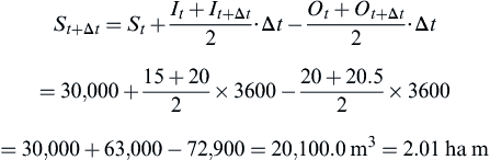
$\begin{matrix} S_{t + Δ t} = S_{t} + \frac{I_{t} + I_{t + Δ t}}{2} \cdot Δ t - \frac{O_{t} + O_{t + Δ t}}{2} \cdot Δ t \\ = 30,000 + \frac{15 + 20}{2} \times 3600 - \frac{20 + 20.5}{2} \times 3600 \\ = 30,000 + 63,000 - 72,900 = 20,100.0 m^{3} = 2.01 ha m \end{matrix}$ $\begin{matrix} S_{t + Δ t} = S_{t} + \frac{I_{t} + I_{t + Δ t}}{2} \cdot Δ t - \frac{O_{t} + O_{t + Δ t}}{2} \cdot Δ t \\ = 30,000 + \frac{15 + 20}{2} \times 3600 - \frac{20 + 20.5}{2} \times 3600 \\ = 30,000 + 63,000 - 72,900 = 20,100.0 m^{3} = 2.01 ha m \end{matrix}$

The change in storage, ΔS = S_t+Δt − S_t = 20,100 − 30,000 = −9900 m³

The storage at the end of the hour is less than the initial storage.

Example 4.8:

The initial storage in the river reach is 2.5 ha m at a given time. Determine the storage at the end of the day. The mean values of inflow and outflow of the reach for the day are 25.0 and 23.5 m³/s, respectively. Also determine the average rise/fall in the river having an area of 10 ha.

Solution:

The hydrologic water budget equation for this problem is given by

$S_{t + Δ t} = S_{t} + \bar{I} \cdot Δ t - \bar{O} \cdot Δ t$ $S_{t + Δ t} = S_{t} + \bar{I} \cdot Δ t - \bar{O} \cdot Δ t$

where S_t = 2.5 ha m = 25,000 m³, Ῑ = 25.0 m³/s,

\bar{O} = 23.5 m^{3} /s

$\bar{O} = 23.5 m^{3} /s$

, Δt = 24 h = 86,400 s. Substituting these values in the above equation we get,

$\begin{matrix} S_{t + Δ t} = S_{t} + \bar{I} \cdot Δ t - \bar{O} \cdot Δ t = 25,000 + 25.0 \times 86,400 - 23.5 \times 86,400 \\ = 154,600 m^{3} = 15.46 ha m \end{matrix}$ $\begin{matrix} S_{t + Δ t} = S_{t} + \bar{I} \cdot Δ t - \bar{O} \cdot Δ t = 25,000 + 25.0 \times 86,400 - 23.5 \times 86,400 \\ = 154,600 m^{3} = 15.46 ha m \end{matrix}$

The average rise in water level in the river is calculated as:

$Δ h = \frac{Δ S}{A_{C}} = \frac{S_{t + Δ t} - S_{t}}{A_{C}} = \frac{15.46 - 2.5}{10} = 1.296 m$ $Δ h = \frac{Δ S}{A_{C}} = \frac{S_{t + Δ t} - S_{t}}{A_{C}} = \frac{15.46 - 2.5}{10} = 1.296 m$

..................Content has been hidden....................

You can't read the all page of ebook, please click here login for view all page.

Table of Contents for 4.3. Hydrologic Equation and Water Balance

Create new playlist

Sign In

Sign Up

4.3. Hydrologic Equation and Water Balance

4.3.1. Period of Water-Balance Exercise

4.3.2. Purpose of Water Balance

Table of Contents for
4.3. Hydrologic Equation and Water Balance