The cropping pattern plays an important role in planning an irrigation project as it decides the water requirement and, ultimately, the capacity of the reservoir and canal system. Selection of crop, based on water availability, climate, soil, affinity, market, income, etc., following the existing cropping pattern should be adequately considered during planning. In addition, selection of optimal crop is important to improve the utilization potential of the existing irrigation projects. Considering the importance of the subject, this chapter describes the procedure of selecting an optimal cropping pattern for the irrigation command using the linear programming technique. It also includes conjunctive-use planning in the command area.
Keywords
Conjunctive use; Cropping pattern; Irrigation potential; Linear programming; Optimal crop planning; Water productivity
Selection of cropping pattern plays an important role while planning an irrigation project, which decides the water requirement at the head and ultimately helps in the estimation of required capacity of the reservoir and the canal system. Selection of crop, based on water availability, climate, soil, affinity, market, income, etc., following the existing cropping pattern, should be adequately considered while planning. In addition, optimal cropping pattern is also important for increased demands of agricultural products, due to population growth, under limited water availability. It also helps in the effective utilization of water and land resources, and improves the water productivity and water-use efficiency of the system. In the agricultural sector, many crops cultivated in a particular region are not suitable for that region. For example, rice and sugarcane are being cultivated in semi-arid regions. In view of this, optimal cropping pattern for planning a sustainable irrigation project is highly required.
In addition, significant deviation in the cropping pattern also affects the existing irrigation projects resulting into reduced irrigation intensity and project duty. For example, the irrigation project in a semi-arid region designed for a cropping pattern comprising 35% wheat crop will in due course result in an uneven supply of water in the command area, if the wheat-cropped area is increased up to 50%–70%. Such deviations in the cropping pattern also reduce the utilization of actual irrigation potential of the designed system. Keeping these considerations in view, it is necessary to identify an optimal cropping pattern for a particular project under various irrigation water availability constraints (i.e., dependable water yield of the project).
An optimal cropping pattern is the allocation of the cropped area with different crops to the culturable command with maximum return for the available water stored in the reservoir. To achieve this, groups of farmers, Water Users Associations (WUAs) or project authority decide the optimum cropping pattern for the command area in the beginning of the season, depending upon the water availability in the reservoir, with the objective of meeting the maximum irrigation potential as well as the maximum economic return. To arrive at an efficient solution of these problems, mathematical models and irrigation management methodologies can be integrated for optimum utilization of resources. For this purpose, linear programming (LP) can be efficiently used. This approach is widely used in the previous studies for achieving different objectives (Loucks et al., 1981; Kumar and Pathak, 1989; Vedula and Mujumdar, 1992; Sethi et al., 2002; Raju and Kumar, 2004). This chapter presents an application of LP as a tool for optimum cropping pattern for the irrigation project under available live storage capacity of the irrigation reservoir.
11.1. Linear Programming
If the objective function and constraints of an optimization model are all linear, then the LP procedure can be applied for planning. In spite of its power and popularity, for most real-time water resources planning and management problems, LP is best viewed as a preliminary tool. Like other optimization methods, LP can provide initial design and operating policy information that simulation models require before they can simulate design and operating policies. The general structure of an LP model is given as follows (Eqs. 11.1–11.3):
MaxorMinz=∑nj=1cjxj
(11.1)
subject to:
∑nj=1aijxj≤bi,fori=1,2,…,m
(11.2)
xj≥0,forallj=1,2,…,n
(11.3)
If any model fits this general form, where the constraints can be any combination of equalities (=) and inequalities (≥ or ≤), LP algorithm can be used to find the “optimal” values of unknown decision variables (i.e., xj).
11.2. LP Formulation for Optimal Crop Planning
The development of an LP model to investigate the optimal cropping pattern is explained further using the following variables:
1. Culturable command area (CCA): A
2. Number of crops sown in the CCA for the crop calendar year, n: 4
3. Type of Rabi crops: wheat, mustard, green gram, and barley
4. Available water in the reservoir for irrigation supply: S
5. System efficiencies: η
6. Irrigation water requirement, average yield, and price of crops
In this formulation, it is assumed that the net input (expenses) is proportional to net return, and the minimum support price (MSP) for the crops is based on the average yield, average return, and average expenses incurred on the crop.
The LP problem for optimal cropping pattern can be formulated as follows (Eq. 11.4):
Objective function:
Maxz=α×∑ni=1YiMSPiAi|Rabi+β×∑mj=1YjMSPjAj∣∣Kharif
(11.4)
where i is the index for the number of Rabi crops; j is the index for the number of Kharif crops; Y is the average yield of the crop (kg/ha); MSP is the minimum support price of the crop (Rs/kg); A is the area under crop (ha); and α and β are the integer values for Rabi and Kharif seasons, respectively. For priority crops such as Kharif protection, value of β should be kept high enough as compared to the value of α.
The conveyance and field efficiency of the system can be considered appropriately based on the condition of conveyance system and irrigation method, respectively.
Subject to constraints:
1. Water availability constraint
∑ni=1[10−5(Ai×CWRi)]≤ηc⋅ηf⋅S
(11.5)
where CWR is the crop water requirement during the growing period of crop (mm); ηc is the conveyance efficiency; ηf is the field application efficiency; and S is the water availability for irrigation supply (MCM).
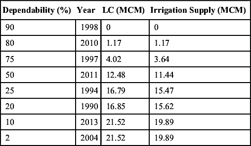
The water available for irrigation supply is computed from the net catchment yield or reservoir yield, by deducting evaporation and seepage losses from the reservoir during the irrigation season. Since optimal cropping pattern is identified under various scenarios of water availability, the dependable reservoir yield term is used. The effective reservoir yield from the most dry to most wet year is considered; in terms of dependable reservoir yield, the 2%, 10%, 20%, 25%, 50%, 75%, 80%, and 90% dependable year yield is considered.
2. Crop area constraint
∑ni=1Ai≤CCA
(11.6)
where CCA is in ha.
3. Nonnegative constraints
Ai≥0;∀i
(11.7)
4. Crop diversity constraint
Ai≥(fi/100)×CCA;∀i
(11.8)
where fi is the minimum percentage of the crop area required to maintain crop diversity.
The LP problem is solved using the simplex method, which yields the optimal area of crops to be cultivated under the available storage. In this formulation, the cost of production will not be considered to estimate the net return from the production. It will be based on the general assumption that gross return is relative to the cost of production, i.e., higher the cost of production, higher will be the gross income and vice versa. CWR can be replaced with the net irrigation requirement (IWRnet) after deducting effective rainfall (ER) from CWR.
To solve these problems easier, “Solver” of MS Excel can be used.
Example 11.1:
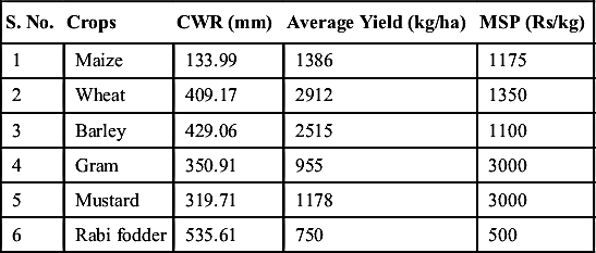
Determine the optimal cropping pattern for the irrigation project having CCA and ICA as 4395 and 3077ha, respectively. The project is designed to irrigate Rabi crops as well as protect Kharif crop during its maturity. The crops supposed to be grown during Rabi are wheat, barley, gram, mustard, and Rabi fodder; whereas for Kharif protection only maize crop is taken. The CWR for these crops are given as follows:
The field application efficiency, ηf and conveyance efficiency ηc will be assumed as 75% and 85%, respectively. Other important inputs of the formulation are summarized in Table 11.1.
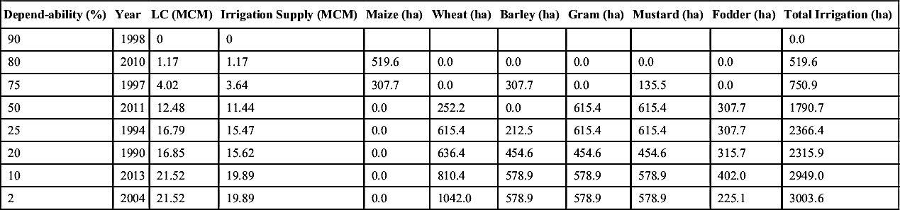
Water availability in the reservoir for various dependable years is given as follows:
Dependability (%)
Year
LC (MCM)
Irrigation Supply (MCM)
90
1998
0
0
80
2010
1.17
1.17
75
1997
4.02
3.64
50
2011
12.48
11.44
25
1994
16.79
15.47
20
1990
16.85
15.62
10
2013
21.52
19.89
2
2004
21.52
19.89
Table 11.1
Basic Input Required for Estimating Optimal Cropping Pattern
S. No.
Crops
CWR (mm)
Average Yield (kg/ha)
MSP (Rs/kg)
1
Maize
133.99
1386
1175
2
Wheat
409.17
2912
1350
3
Barley
429.06
2515
1100
4
Gram
350.91
955
3000
5
Mustard
319.71
1178
3000
6
Rabi fodder
535.61
750
500
Solution:
The LP formulation is developed on MS Excel to use the “Solver” program as follows. The basic input is prepared and summarized in Table 11.2.
CCA=4395ha; ICA=3077ha.
Case I: Optimal cropping pattern for 80% dependable year yield (S=1.17MCM):
Basic Input Required for Estimating the Optimal Cropping Pattern
Components
Maize
Wheat
Barley
Gram
Mustard
Fodder
Total
CWR (mm)
133.99
409.17
429.06
350.91
319.71
535.61
GIR (mm)
225.19
687.68
721.11
589.76
537.32
900.18
Area under crop (ha)
?
?
?
?
?
?
?
Cropping pattern
?
?
?
?
?
?
Average yield (kg/ha)
1386
2912
2515
955
1178
750
MSP (Rs/qt)
1175
1350
1100
3000
3000
500
Gross return (lakh Rs)
?
?
?
?
?
?
Objective function, z
GIR (MCM)
?
?
?
?
?
?
?
3. Nonnegative constraints
AMaize≥0
AWheat≥0
ABarley≥0
AGram≥0
AMustard≥0
AFodder≥0
4. Crop diversity constraints
AWheat≥30%
ABarley≥5%
AGram≥5%
AMustard≥5%
AFodder≥5%
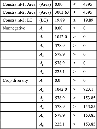
All these constraints are summarized as below:
Constraint-1: Area
(Area)
0.00
≤
4395
Constraint-2: Area
(Area)
3003.63
≤
4395
Constraint-3: LC
(LC)
19.89
≤
19.89
Nonnegative
A1
0.00
>
0
A2
1042.0
>
0
A3
578.9
>
0
A4
578.9
>
0
A5
578.9
>
0
A6
225.1
>
0
Crop diversity
A1
0.0
>
0
A2
1042.0
>
923.1
A3
578.9
>
153.85
A4
578.9
>
153.85
A5
578.9
>
153.85
A6
225.1
>
153.85
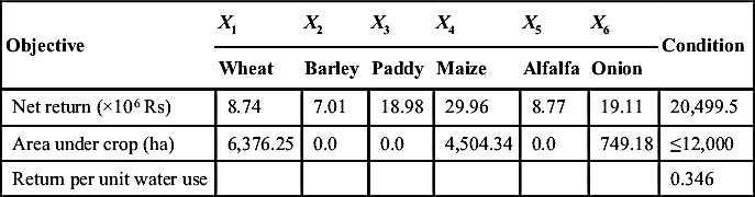
The value of α was considered lower as compared to β for higher value of dependability (i.e., 75%–90%). Solving the LP problem, the following cropping pattern is obtained for 80% dependable year:
Solving the above LP problem, the cropping pattern obtained is
Objective
X1
X2
X3
X4
X5
X6
Condition
Wheat
Barley
Paddy
Maize
Alfalfa
Onion
Net return (×106Rs)
8.74
7.01
18.98
29.96
8.77
19.11
20,499.5
Area under crop (ha)
6,376.25
0.0
0.0
4,504.34
0.0
749.18
≤12,000
Return per unit water use
0.346
Example 11.3:
Irrigation in the agricultural land is being met by run-of-river diversion project having mean monthly inflow as given below. The CCA of the area diversion scheme is 600ha for which the cropping pattern need to be optimized between three crops, namely wheat, alfalfa, and cotton, having a net water demand as given below. Assume irrigation efficiency to be 65%. Also, determine the monthly diversion or water allocation.
Month
Monthly Inflow, I (m3/s)
Net Water Demand (mm)
Wheat
Alfalfa
Cotton
Sep.
0.20
0
0
114
Oct.
0.35
14.0
14.0
61
Nov.
1.00
5.0
5.0
Dec.
1.50
4.0
5.0
Jan.
1.70
2.0
1.0
Feb.
0.80
1.5
2.0
Mar.
0.75
33.0
33.0
Table Continued
Month
Monthly Inflow, I (m3/s)
Net Water Demand (mm)
Wheat
Alfalfa
Cotton
Apr.
0.60
142.0
141.0
24
May
0.36
138.0
97.0
82
Jun.
0.25
2.0
0
190
Jul.
0.20
0
0
225
Aug.
0.15
0
0
186
Total
341.5
298.0
882.0
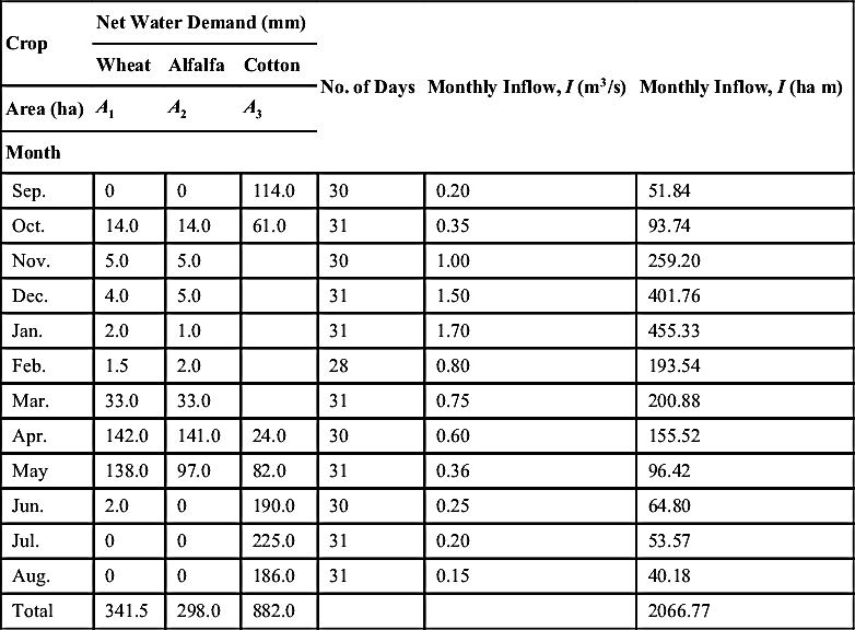
Solution:
The LP formulation will be as follows.
Let A1, A2, and A3 be the areas under wheat, alfalfa, and cotton crops. Before proceeding further into the LP formulation the following computations are to be made:
Crop
Net Water Demand (mm)
No. of Days
Monthly Inflow, I (m3/s)
Monthly Inflow, I (ha m)
Wheat
Alfalfa
Cotton
Area (ha)
A1
A2
A3
Month
Sep.
0
0
114.0
30
0.20
51.84
Oct.
14.0
14.0
61.0
31
0.35
93.74
Nov.
5.0
5.0
30
1.00
259.20
Dec.
4.0
5.0
31
1.50
401.76
Jan.
2.0
1.0
31
1.70
455.33
Feb.
1.5
2.0
28
0.80
193.54
Mar.
33.0
33.0
31
0.75
200.88
Apr.
142.0
141.0
24.0
30
0.60
155.52
May
138.0
97.0
82.0
31
0.36
96.42
Jun.
2.0
0
190.0
30
0.25
64.80
Jul.
0
0
225.0
31
0.20
53.57
Aug.
0
0
186.0
31
0.15
40.18
Total
341.5
298.0
882.0
2066.77
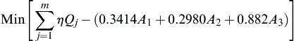
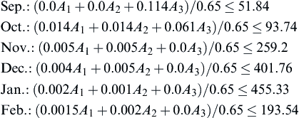
Let Qj be the monthly allocation of water to the agricultural land having a total CCA of 600ha. The objective function will be defined as to satisfy the gross irrigation requirement on the field, considering the scheme irrigation efficiency of 65%.
Min[∑mj=1ηQj−(0.3414A1+0.2980A2+0.882A3)]
where j is the index for the month and m is number of months during the irrigation season.
Figure 11.1 Monthly inflow and diversion from head work for irrigating crops.
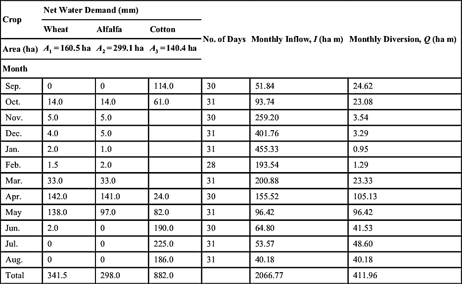
Solving the above LP problem, the areas under wheat (A1), alfalfa (A2), and cotton (A3) are determined as 160.5, 299.1, and 140.4ha, respectively. The water to be diverted for irrigation in each month will be (Fig. 11.1):
Crop
Net Water Demand (mm)
No. of Days
Monthly Inflow, I (ha m)
Monthly Diversion, Q (ha m)
Wheat
Alfalfa
Cotton
Area (ha)
A1=160.5ha
A2=299.1ha
A3=140.4ha
Month
Sep.
0
0
114.0
30
51.84
24.62
Oct.
14.0
14.0
61.0
31
93.74
23.08
Nov.
5.0
5.0
30
259.20
3.54
Dec.
4.0
5.0
31
401.76
3.29
Jan.
2.0
1.0
31
455.33
0.95
Feb.
1.5
2.0
28
193.54
1.29
Mar.
33.0
33.0
31
200.88
23.33
Apr.
142.0
141.0
24.0
30
155.52
105.13
May
138.0
97.0
82.0
31
96.42
96.42
Jun.
2.0
0
190.0
30
64.80
41.53
Jul.
0
0
225.0
31
53.57
48.60
Aug.
0
0
186.0
31
40.18
40.18
Total
341.5
298.0
882.0
2066.77
411.96
11.3. LP-Based Conjunctive Use of Surface and Groundwater Resources
Conjunctive use implies a planned and coordinated management of surface and groundwater resources to maximize the efficient use of total water resources. Subsurface water can be used as a supplement to surface water during dry periods and peak demand periods as well as during periods of low rainfall. However, the conjunctive use of both surface water and subsurface water can avoid the overexploitation of any of these two resources. Optimization techniques could be very useful tool for conjunctive-use modeling. In this section, we will describe the conjunctive-use modeling using LP.
To start with, let us divide the total time duration (normally a water year) into discrete periods. The temporal resolution is problem specific and it could be in days, weeks, or months, or seasons like Rabi, Kharif, etc. Let us assume that we have M discrete periods. Also, assume that we have N feasible crops in the command area.
11.3.1. Decision Variables
For the conjunctive-use modeling the decision variables are:
1. Area of all feasible crops Aj; j=1, 2, 3,…, N in ha.
2. Canal release QCk; k=1, 2, 3, …, M in ham.
3. Groundwater withdrawal QGk; k=1, 2, 3, …, M in ham.
11.3.2. Objective Function
In this case, we have taken the objective function as the maximization of net benefit from agricultural activity. However, the objective function depends upon the problem at hand. The net benefit would be the total market return minus the total cost of input. The cost of input here is divided into three sections: the cost of canal water, the cost of groundwater, and the cost other than that of water, which may include other expenditures, such as seeds, fertilizers, labor, transportation, etc. The objective function can be written as Eq. (11.9).
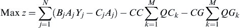
Maxz=∑Nj=1(BjAjYj−CjAj)−CC∑Mk=1QCk−CG∑Mk=1QGk
(11.9)
We can see from the objective function equation that it is a linear function of decision variables.
Bj is the market return for the jth crop in Rs/ton; Yj is the yield per hectare for jth crop in ton/ha; Cj is the cost of input other than that of water in Rs/ha; CC is the cost of unit volume of canal water in Rs/ham; and CG is the cost of unit volume of groundwater in Rs/ham.
11.3.3. Constraints
The LP problem cannot be unconstrained; however, in this case, crop area, canal release, and groundwater withdrawals are the decision variables. Therefore the constraints are to be imposed to restrict excessive mining of these resources. The following constraints are used.
11.3.3.1. Water Availability Constraint
This constraint states that the total irrigation water requirement should be less than or equal to the available water. For the kth period, where k=1, 2, 3, …, M, the constraint can be written as Eq. (11.10).
∑Nj=1(Ajδjk)≤ηcQCk+ηgQGk
(11.10)
where δjk is the irrigation water requirement for jth in m for kth period, ηc and ηg are the conveyance efficiency w.r.t. canal water and groundwater, respectively. We would have one constraint for each period; therefore we would have total M such constraints.
11.3.3.2. Land Availability Constraint
This constraint states that the total area occupied by crops at any time period should be less than the CCA or actual area available for agriculture during that period. For the kth period where k=1, 2, 3, …, M, the constraint can be written as Eq. (11.11)
∑Nj=1(Ajθjk)≤CCA
(11.11)
where θjk is the area occupied by one unit area of the jth in the kth period. Its value varies from 0 to 1: 0 when the crop is absent and 1 when the crop is present.
11.3.3.3. Crop Area Limits
There could be a constraint on the maximum and minimum permissible areas under any crop. This constraint can be written as Eq. (11.12).
Amaxj≥Aj≥Aminj;j=1,2,3,…,N
(11.12)
11.3.3.4. Surface Water–Resources Constraint
There could be constraints on the maximum water that can be released from the canal (Eqs. 11.13 and 11.14).
QCk≤Canalconveyancecapacity
(11.13)
∑mk=1QCk≤Reservoircapacityallocatedtoirrigation
(11.14)
where k=1, 2, 3, …, m; and m is number of season or period (in months).
11.3.3.5. Groundwater Resources Constraint
This constraint restricts the maximum and minimum amount of water that can be withdrawn from the groundwater source. A certain minimum quantity of water is to be withdrawn from the groundwater to avoid water logging in the area. On the contrary, the water withdrawn from the groundwater should not lead to excessive lowering of water table. This constraint is written as Eq. (11.15).
ηg∑mk=1QGk≥PGW
(11.15)
On the contrary, the water withdrawn from groundwater should not lead to excessive lowering of the water table. This constraint is written as Eq. (11.16).
ηˆg∑mk=1QGk≤PGW+M
(11.16)
where PGW is post-project groundwater resource in ham; M is the permissible mining in ham; and ηˆg is the overall efficiency in respect to groundwater.
Example 11.4:
In an area of 170sq. km having CCA of 80%, three feasible crops, namely wheat, sugarcane, and paddy, are grown. The annual surface water available and annual groundwater recharges are 5000 and 2000ham, respectively. Recharge from the canal system is 20% of the annual canal water release. The net benefits (excluding cost of water) in Rs/ha for wheat, sugarcane, and paddy are 4000, 9500, and 2150Rs/ha, respectively. The cost of groundwater and cost of canal water are Rs. 1000 and Rs. 650/ham. The maximum permissible areas for wheat, sugarcane, and paddy are 5800, 7500, and 5200ha, respectively.
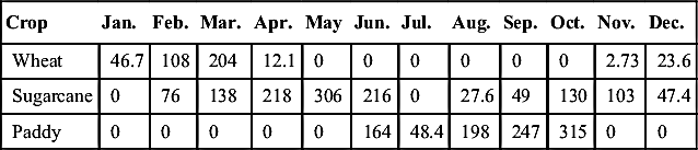
The irrigation efficiency for groundwater and canal water are 0.8 and 0.6, respectively. The canal conveyance capacity is 750ham/month and the maximum permissible monthly pumpage is 700ham. The net irrigation requirement (mm) is
Crop
Jan.
Feb.
Mar.
Apr.
May
Jun.
Jul.
Aug.
Sep.
Oct.
Nov.
Dec.
Wheat
46.7
108
204
12.1
0
0
0
0
0
0
2.73
23.6
Sugarcane
0
76
138
218
306
216
0
27.6
49
130
103
47.4
Paddy
0
0
0
0
0
164
48.4
198
247
315
0
0
Compute the optimal conjunctive-use policy using LP, which maximizes the net benefit.
Solution:
Let A1, A2, and A3 be the areas under wheat, sugarcane and paddy, respectively. The above LP problem can be written as follows.
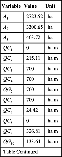
The above problem contains 43 constraints and 28 decision variables. Therefore this problem is solved using Lindo, and the final solution obtained is provided in Table 11.3.
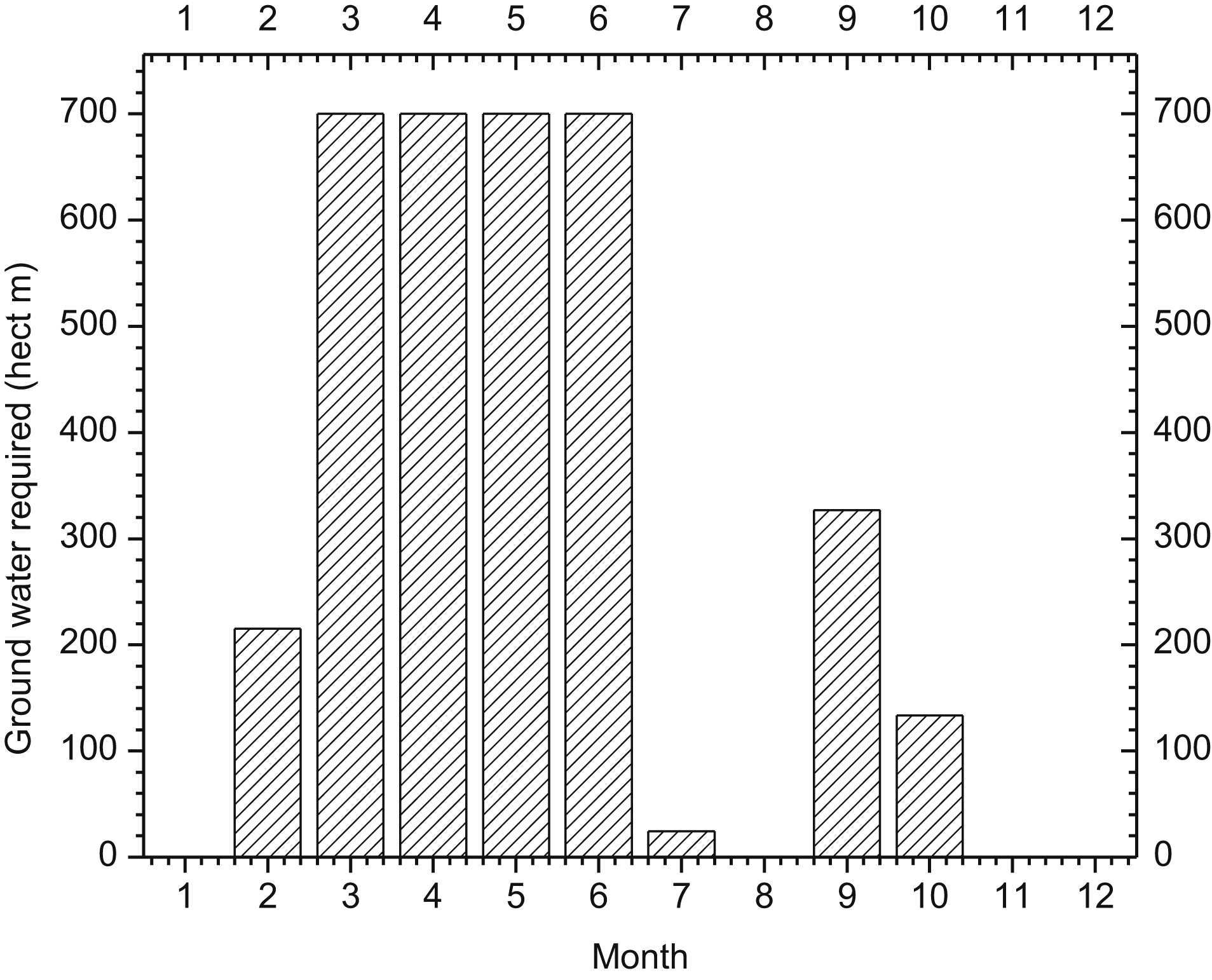
It can be seen from Figs. 11.2 and 11.3 that there would be more dependency on groundwater in the nonmonsoon periods, i.e., from October to June. From October to January more utilization of surface water resources takes place, whereas from March to June maximum utilization of both surface and groundwater resources takes place (Figs. 11.2 and 11.3).
Figure 11.2 Monthwise groundwater required.
Figure 11.3 Monthwise canal water required.
Table 11.3
Optimal Values of Decision Variables in Example 11.4
Variable
Value
Unit
A1
2723.52
ha
A2
3300.65
ha
A3
403.72
ha
QG1
0
ha m
QG2
215.11
ha m
QG3
700
ha m
QG4
700
ha m
QG5
700
ha m
QG6
700
ha m
QG7
24.42
ha m
QG8
0
ha m
QG9
326.81
ha m
QG10
133.64
ha m
Table Continued
Variable
Value
Unit
QG11
0
ha m
QG12
0
ha m
QC1
211.98
ha m
QC2
619.68
ha m
QC3
750
ha m
QC4
321.01
ha m
QC5
750
ha m
QC6
365.38
ha m
QC7
0
ha m
QC8
285.05
ha m
QC9
0
ha m
QC10
750
ha m
QC11
579.00
ha m
QC12
367.87
ha m
11.4. Concluding Remarks
The chapter discusses optimal crop planning for irrigation projects using the LP technique, considering necessary constraints like water availability, crop types, crop affinity, financial cost and benefits, etc., with the ultimate objective of maximizing the net return, equitable distribution of water, and water-use efficiency. The chapter also includes the conjunctive-use planning in the command area.
 (11.1)
 (11.2)
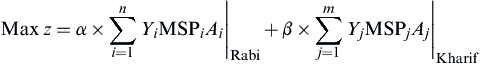 (11.4)
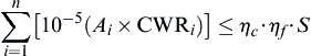 (11.5)
 (11.6)
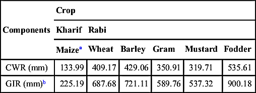


 (11.9)
 (11.10)
 (11.11)
 (11.14)
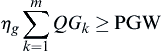 (11.15)
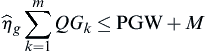 (11.16)