4.6. Inflow Estimation in Multi-Reservoir Case

Search in book...
Toggle Font Controls
Create new playlist

Name your new playlist

Playlist description (optional)
Sign In

Email address

Password

Forgot Password?

or

Continue with Facebook

Continue with Google
Sign Up

Full Name

Email address

Confirm Email Address

Password

or

Continue with Facebook

Continue with Google

4.6. Inflow Estimation in Multi-Reservoir Case

In many cases, multiple reservoirs are constructed in the catchment for distributed water supply; under such a situation the modeling framework used to simulate the inflow at the outlet of the catchment is presented in Fig. 4.7.

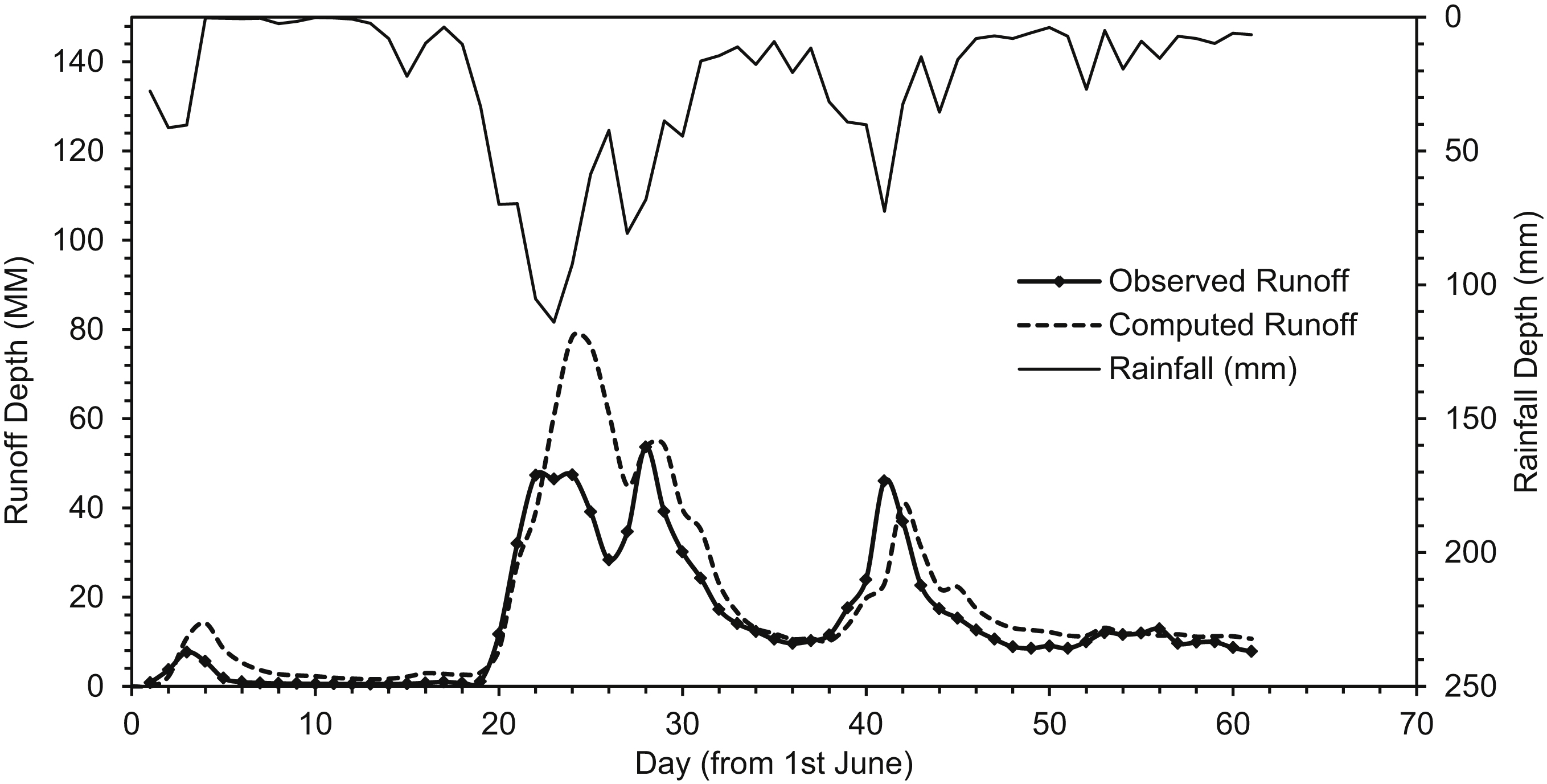
Figure 4.6 Comparison of observed and computed runoff hydrograph by Modified SCS-CN method.

Figure 4.7 Schematic presentation of multi-reservoirs in the catchment.

The steps followed in the estimation of inflow hydrograph for the last reservoir using the uncoupled modeling approach are as follows:

Step I: Determine the inflow hydrograph for reservoirs 1 and 2 (i.e., R1 and R2) using the catchment water-balance approach or modified SCS-CN method for catchments C1 and C2.

Step II: Compute the runoff hydrograph from catchment C3 (i.e., total intermediate catchments).

Step III: Carry out the reservoir routing to estimate the outflow from reservoirs R1 and R2 using the storage-indication method described in the following section. The reservoir overflow equation is used to estimate the overflow discharge. If spillway rating curve function is not available for the projects then appropriate overflow spillway or sluice flow equation is used.

Step IV: The outflows generated from the two upstream reservoirs are combined and subjected to the channel routing using the Muskingum method. For channel routing, the runoff generated from catchment C3 (Step II) is uniformly distributed to the channel. Details of the Muskingum method of channel routing are described in following section.

Step V: The resulting hydrograph from channel routing will be the inflow hydrograph for reservoir R3.

4.6.1. Reservoir Routing: Storage-Indication Method

The storage-indication method is also known as the modified pulse method or level pool method, which is used for reservoir routing (SCS, 1972; Singh, 1988; Chow et al., 1988). This method can also be used for channel routing through actual reservoirs for which the storage–discharge relationship is usually nonlinear. This method will also be useful for determining the maximum water level (MWL) for the reservoir with design flood as inflow.

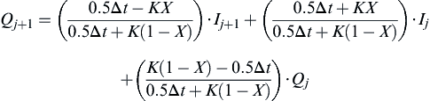
Again, the hydrologic continuity equation is used to derive the governing equation for the storage-indication method. Expanding and rearranging the terms in Eq. (4.43), the following equation is obtained:

$(I_{j} + I_{j + 1}) - (O_{j} + O_{j + 1}) = \frac{2 S_{j + 1}}{Δ t} - \frac{2 S_{j}}{Δ t}$ $(I_{j} + I_{j + 1}) - (O_{j} + O_{j + 1}) = \frac{2 S_{j + 1}}{Δ t} - \frac{2 S_{j}}{Δ t}$

(4.68)

$(\frac{2 S_{j + 1}}{Δ t} + O_{j + 1}) = (I_{j} + I_{j + 1}) + (\frac{2 S_{j}}{Δ t} - O_{j})$ $(\frac{2 S_{j + 1}}{Δ t} + O_{j + 1}) = (I_{j} + I_{j + 1}) + (\frac{2 S_{j}}{Δ t} - O_{j})$

(4.69)

Eq. (4.68) is the governing equation for the storage-indication method. In Eq. (4.69), S_j+1 and O_j+1 are the two unknown values on the left hand side. The term [(2S_j+1/Δt) + O_j+1] is referred to as the storage-indication function. Therefore while using the storage-indication method, it is a prerequisite to derive the elevation–storage curve, elevation–discharge curve, and storage-indication function–discharge curve. The steps involved in using the storage-indication method are as follows:

1. Examine the topography of the reservoir-elevation and storage-characteristic data (i.e., elevation-capacity table).

2. Collect the spillway information to develop an elevation–discharge relationship. It should also include the reservoir operation rule.

3. Derive the storage indication–discharge relationship [(2S_j+1/Δt) + O_j+1] using the derived information from Steps (2) and (3).

4. Create an operational table for computations:

a. Arrange the incremental time in Col. 1.

b. Arrange the inflow hydrograph ordinates corresponding to the time in Col. 2.

c. Determine term (I_j + I_j+1) and arrange the values in Col. 3.

d. Determine term [(2S_j/Δt) − O_j] using the recursive relationship and arrange in Col. 4 as follows:

$(\frac{2 S_{j}}{Δ t} - O_{j}) = (\frac{2 S_{j}}{Δ t} + O_{j}) - 2 O_{j}$ $(\frac{2 S_{j}}{Δ t} - O_{j}) = (\frac{2 S_{j}}{Δ t} + O_{j}) - 2 O_{j}$

(4.70)

e. Determine term [(2S_j+1 /Δt) + O_j+1] using Eq. (4.68) and arrange in Col. 5.

f. Determine O_j+1 corresponding to the storage-indication function, [(2S_j+1 /Δt) + O_j+1] derived in Step (4) and arrange in Col. 6. The corresponding discharge is estimated either graphically or using the linear interpolation technique.

g. Repeat Steps (a) to (f) until routing is over.

Data requirement: (1) Elevation–capacity curve or table; (2) rating curve or elevation–discharge relationship for the weir; (3) inflow hydrograph; and (4) operation rule or diversion rule for water supply.

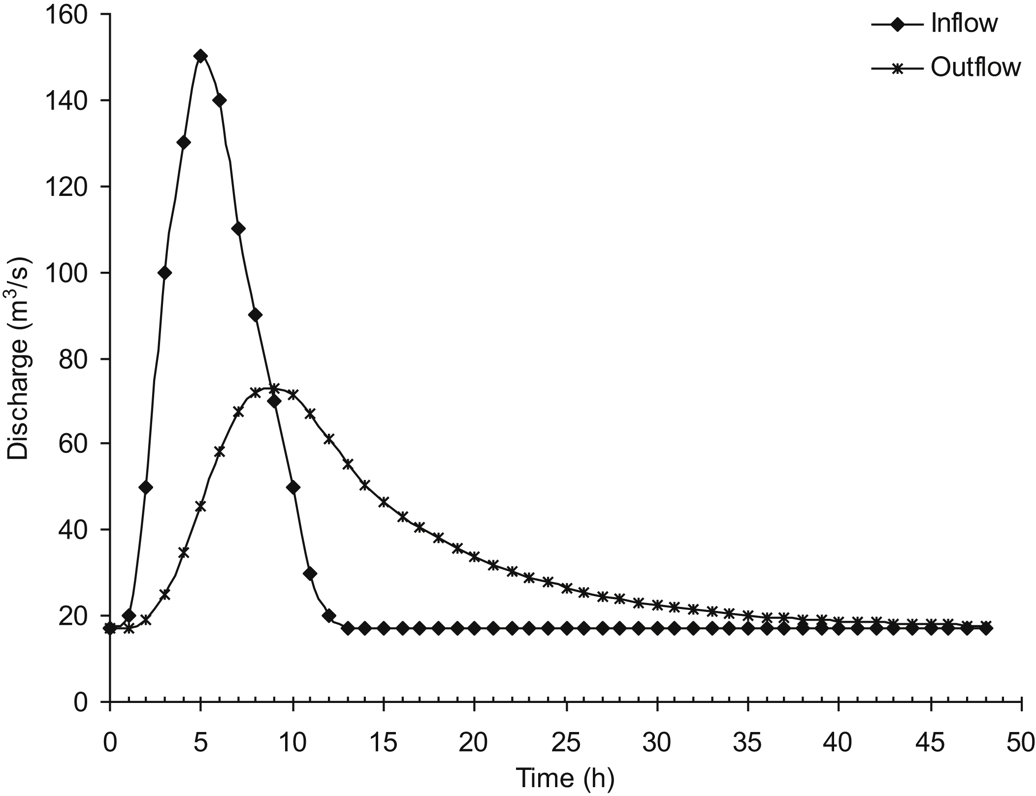
Example 4.11:

The design of an emergency spillway calls for a broad-crested weir of width L = 10.0 m; rating coefficient C_d = 1.70; and exponent y = 1.5. The spillway crest is at an elevation 1070 m. Above this level, the reservoir walls can be considered to be vertical, with a surface area of 100 ha. The dam crest is at an elevation of 1076 m. Baseflow is 17 m³/s, and the initial reservoir level is 1071 m. Route the following design hydrograph through the reservoir.

Time (h)	1	2	3	4	5	6	7	8
Inflow (m³/s)	20	50	100	130	150	140	110	90
Time (h)	9	10	11	12	13	14	15	16
Inflow (m³/s)	70	50	30	20	17	17	17	17

What is the maximum pool elevation or MWL reached? Assume the reservoir surface area between elevations of 1070 and 1076 m is 100 ha.

Solution:

The following steps are considered in reservoir routing using the storage-indication method:

(i) Derive the spillway-rating relationship using the following equation:

$Q = C_{d e s} L {(H_{d e s} - Δ z)}^{y}$ $Q = C_{d e s} L {(H_{d e s} - Δ z)}^{y}$

$Q = 1.70 \times 10 \times {(H_{d e s} - 1070)}^{1.5} = 17.0 {(H_{d e s} - 1070)}^{1.5}$ $Q = 1.70 \times 10 \times {(H_{d e s} - 1070)}^{1.5} = 17.0 {(H_{d e s} - 1070)}^{1.5}$

(ii) Derive the relationships between the elevation–storage, the elevation–discharge, and the storage–indication function as follows (Table 4.18):

Col. 2 = Col. 1 − Spillway crest elevation

Col. 3 = 17.0 × (Col. 2)^1.5

Since reservoir is vertical above an elevation of 1070 m, Col. 4: Reservoir area × Col. 2 = 1,000,000 × Col. 2 (m³)

The storage-indication function is calculated and arranged in Col. 5 as follows:

Col. 5 = [(2 × Col. 4)/(Δt × 3600)] + Col. 3; where Δt = 1 h.

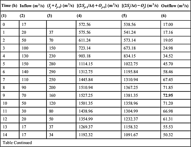
(iii) Create the routing computation table as follows (Table 4.19):

(a) Arrange the time and inflow ordinates in Cols. 1 and 2, respectively.

(b) Compute term (I_j + I_j+1) and arrange in Col. 3. For t = 1 h, I_j + I_j+1 = 17 + 20 = 37 m³/s.

(c) Provide the initial condition of discharge equal to baseflow (i.e., 17 m³/s), and the corresponding value of storage–indication function from the above table (i.e., 572.56 m³/s) in Cols. 6 and 4, respectively.

(d) Compute term [(2S_j/Δt) − O_j] as follows (Col. 5):

$(\frac{2 S_{j + 1}}{Δ t} - O_{j + 1}) = (\frac{2 S_{j + 1}}{Δ t} + O_{j + 1}) - 2 O_{j + 1}$ $(\frac{2 S_{j + 1}}{Δ t} - O_{j + 1}) = (\frac{2 S_{j + 1}}{Δ t} + O_{j + 1}) - 2 O_{j + 1}$

For t = 0, Q = 17 m³/s, [(2S_j+1/Δt) + O_j+1] = 572.56 m³/s, then [(2S_j=0/Δt) − O_j=0] = [(2S_j=0/Δt) + O_j=0] − 2O_j=0 = 538.56 m³/s.

(e) Compute the storage-indication function for the next time step and arrange in Col. 4. For time step, t=2 h, [(2S_t=1/Δt) + O_t=1] = (I_t=0 + I_t=1) + [(2S_t=0/Δt) − O_t=0] = 37 + 538.56 = 575.56 m³/s.

(f) Compute the spillway discharge corresponding to [(2S_t=1/Δt) + O_t=1] using the linear interpolation technique as:

$y = y_{1} + \frac{y_{2} - y_{1}}{x_{2} - x_{1}} \cdot (x - x_{1})$ $y = y_{1} + \frac{y_{2} - y_{1}}{x_{2} - x_{1}} \cdot (x - x_{1})$

For t = 1 h, [(2S_t=1/Δt) + O_t=1] = 575.56 m³/s.

Then

O_{t = 1} = 17 + 17.0 + \frac{48.08 - 17.0}{1159.19 - 572.56} \cdot (575.56 - 572.56) = 17.158 \approx 17.16 m^{3} / s

$O_{t = 1} = 17 + 17.0 + \frac{48.08 - 17.0}{1159.19 - 572.56} \cdot (575.56 - 572.56) = 17.158 \approx 17.16 m^{3} / s$

(g) Repeat Steps (d) to (f) until routing is completed.

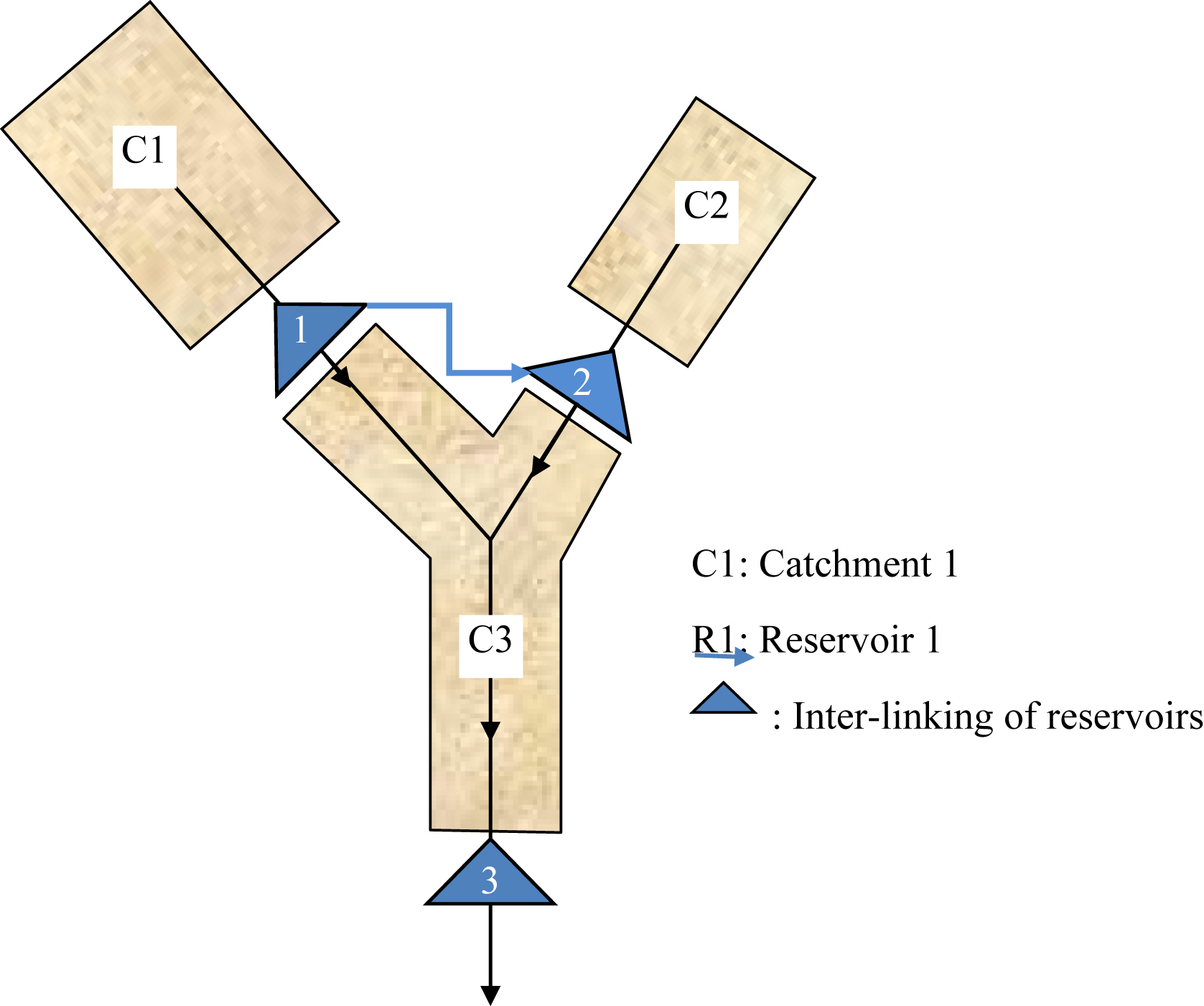
(iv) Determine the maximum pool elevation using the rating curve relationship as follows:

$O_{p} = 17.0 \times {(H_{max \cdot pool} - 1070)}^{1.5}$ $O_{p} = 17.0 \times {(H_{max \cdot pool} - 1070)}^{1.5}$

Solving for H_max·pool yields:

$(H_{\max \cdot pool} - 1070) = {(\frac{72.95}{17.0})}^{1 / 1.5} = 2.6407 m$ $(H_{\max \cdot pool} - 1070) = {(\frac{72.95}{17.0})}^{1 / 1.5} = 2.6407 m$

Therefore H_max·pool = 1070 + 2.6407 = 1072.6407 m.

(v) Examine the inflow and outflow hydrograph through visual comparison (Fig. 4.8):

Table 4.18

Derivation of Storage–Indication Function for Example 4.11

Elevation (m)	H_des − Δz (m)	Spillway Discharge (m³/s)	Storage (m³)	Storage-Indication Function [(2S_j+1/Δt) + O_j+1] (m³/s)
(1)	(2)	(3)	(4)	(5)
1070	0	0.00	0	0.00
1071	1	17.00	1,000,000	572.56
1072	2	48.08	2,000,000	1159.19
1073	3	88.33	3,000,000	1755.00
1074	4	136.00	4,000,000	2358.22
1075	5	190.07	5,000,000	2967.84
1076	6	249.85	6,000,000	3583.18

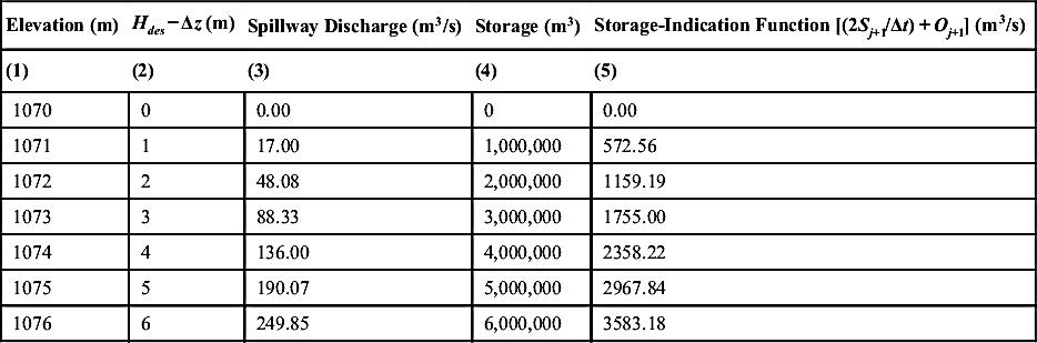
Table 4.19

Reservoir Routing Computation Using Storage—Indication for Example 4.11

Time (h)	Inflow (m³/s)	(I_j + I_j+1) (m³/s)	[(2S_j+1/Δt) + O_j+1] (m³/s)	[(2S_j/Δt) − O_j] (m³/s)	Outflow (m³/s)
(1)	(2)	(3)	(4)	(5)	(6)
0	17		572.56	538.56	17.00
1	20	37	575.56	541.24	17.16
2	50	70	611.24	573.14	19.05
3	100	150	723.14	673.18	24.98
4	130	230	903.18	834.15	34.52
5	150	280	1114.15	1022.75	45.70
6	140	290	1312.75	1195.84	58.46
7	110	250	1445.84	1310.94	67.45
8	90	200	1510.94	1367.25	71.85
9	70	160	1527.25	1381.35	72.95
10	50	120	1501.35	1358.96	71.20
11	30	80	1438.96	1304.99	66.98
12	20	50	1354.99	1232.37	61.31
13	17	37	1269.37	1158.32	55.53
14	17	34	1192.32	1091.67	50.32
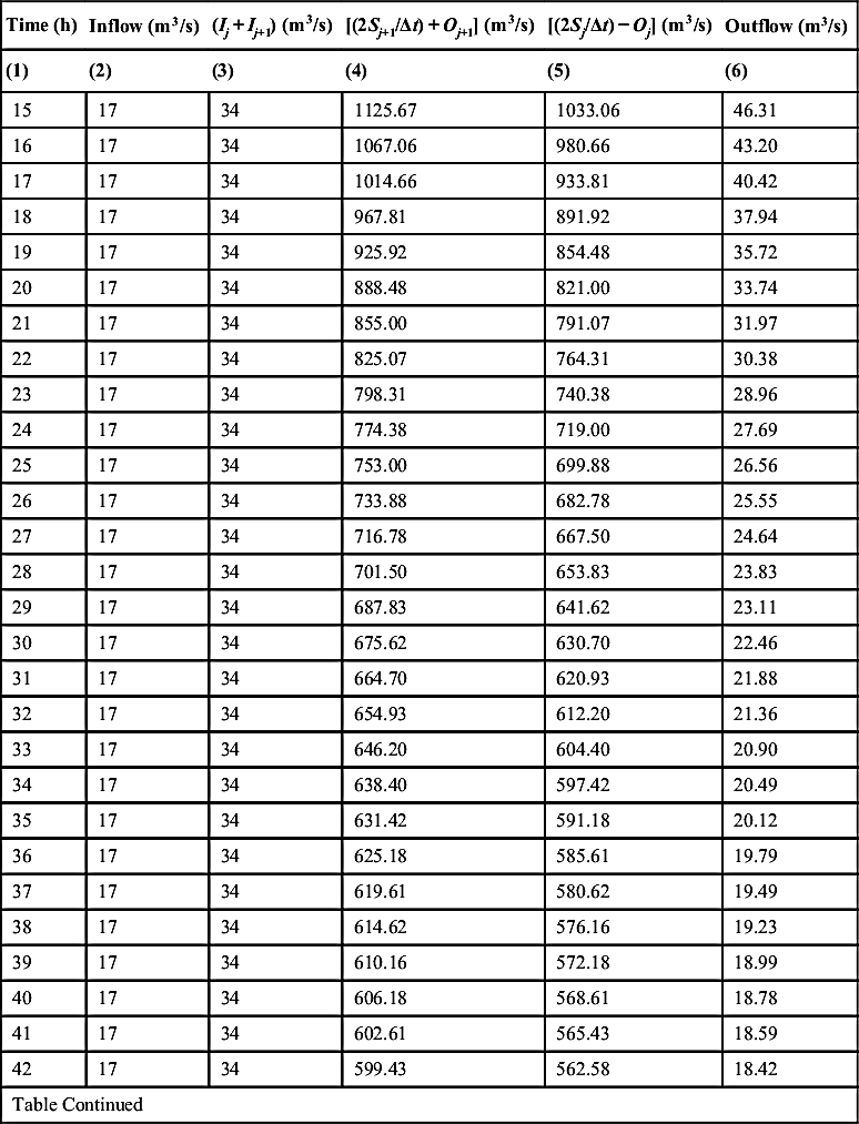
Table Continued

Time (h)	Inflow (m³/s)	(I_j + I_j+1) (m³/s)	[(2S_j+1/Δt) + O_j+1] (m³/s)	[(2S_j/Δt) − O_j] (m³/s)	Outflow (m³/s)
(1)	(2)	(3)	(4)	(5)	(6)
15	17	34	1125.67	1033.06	46.31
16	17	34	1067.06	980.66	43.20
17	17	34	1014.66	933.81	40.42
18	17	34	967.81	891.92	37.94
19	17	34	925.92	854.48	35.72
20	17	34	888.48	821.00	33.74
21	17	34	855.00	791.07	31.97
22	17	34	825.07	764.31	30.38
23	17	34	798.31	740.38	28.96
24	17	34	774.38	719.00	27.69
25	17	34	753.00	699.88	26.56
26	17	34	733.88	682.78	25.55
27	17	34	716.78	667.50	24.64
28	17	34	701.50	653.83	23.83
29	17	34	687.83	641.62	23.11
30	17	34	675.62	630.70	22.46
31	17	34	664.70	620.93	21.88
32	17	34	654.93	612.20	21.36
33	17	34	646.20	604.40	20.90
34	17	34	638.40	597.42	20.49
35	17	34	631.42	591.18	20.12
36	17	34	625.18	585.61	19.79
37	17	34	619.61	580.62	19.49
38	17	34	614.62	576.16	19.23
39	17	34	610.16	572.18	18.99
40	17	34	606.18	568.61	18.78
41	17	34	602.61	565.43	18.59
42	17	34	599.43	562.58	18.42
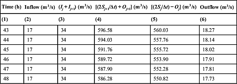
Table Continued

Time (h)	Inflow (m³/s)	(I_j + I_j+1) (m³/s)	[(2S_j+1/Δt) + O_j+1] (m³/s)	[(2S_j/Δt) − O_j] (m³/s)	Outflow (m³/s)
(1)	(2)	(3)	(4)	(5)	(6)
43	17	34	596.58	560.03	18.27
44	17	34	594.03	557.76	18.14
45	17	34	591.76	555.72	18.02
46	17	34	589.72	553.90	17.91
47	17	34	587.90	552.28	17.81
48	17	34	586.28	550.82	17.73

Figure 4.8 Comparison of inflow and outflow hydrograph for Example 4.11.

4.6.2. Channel Routing

4.6.2.1. The Muskingum Method

The Muskingum method is a commonly used hydrologic routing method for channel flow (Nash, 1959; Cunge, 1969; Ponce, 1979; Singh, 1988). It uses the storage–discharge relationship in a river reach by combining wedge and prism storages.

The Muskingum-storage function used in the routing is given by:

$S = K [X I + (1 - X) Q]$ $S = K [X I + (1 - X) Q]$

(4.71)

The value of X ranges from 0 for reservoir-type storage to 0.5 for a full-wedge storage. When X = 0, there is no wedge and hence no back water effect in the channel. In natural streams, X varies between 0 and 0.3 with a mean value near 0.2. Parameter K is the time of travel of the flood wave through the channel reach.

Substituting the term S in discrete form in Eq. (4.37) and thereafter in Eq. (4.36), and rearranging the terms gives the governing equation for the Muskingum-channel routing.

$\begin{matrix} Q_{j + 1} = (\frac{0.5 Δ t - K X}{0.5 Δ t + K (1 - X)}) \cdot I_{j + 1} + (\frac{0.5 Δ t + K X}{0.5 Δ t + K (1 - X)}) \cdot I_{j} \\ + (\frac{K (1 - X) - 0.5 Δ t}{0.5 Δ t + K (1 - X)}) \cdot Q_{j} \end{matrix}$ $\begin{matrix} Q_{j + 1} = (\frac{0.5 Δ t - K X}{0.5 Δ t + K (1 - X)}) \cdot I_{j + 1} + (\frac{0.5 Δ t + K X}{0.5 Δ t + K (1 - X)}) \cdot I_{j} \\ + (\frac{K (1 - X) - 0.5 Δ t}{0.5 Δ t + K (1 - X)}) \cdot Q_{j} \end{matrix}$

(4.72)

For computational ease, Eq. (4.72) can also be expressed as follows:

$Q_{j + 1} = C_{1} \cdot I_{j + 1} + C_{2} \cdot I_{j} + C_{3} \cdot Q_{j}$ $Q_{j + 1} = C_{1} \cdot I_{j + 1} + C_{2} \cdot I_{j} + C_{3} \cdot Q_{j}$

(4.73)

where

$C_{1} = \frac{0.5 Δ t - K X}{0.5 Δ t + K (1 - X)}$ $C_{1} = \frac{0.5 Δ t - K X}{0.5 Δ t + K (1 - X)}$

(4.74)

$C_{2} = \frac{0.5 Δ t + K X}{0.5 Δ t + K (1 - X)}$ $C_{2} = \frac{0.5 Δ t + K X}{0.5 Δ t + K (1 - X)}$

(4.75)

$C_{3} = \frac{K (1 - X) - 0.5 Δ t}{0.5 Δ t + K (1 - X)}$ $C_{3} = \frac{K (1 - X) - 0.5 Δ t}{0.5 Δ t + K (1 - X)}$

(4.76)

$C_{1} + C_{2} + C_{3} = 1$ $C_{1} + C_{2} + C_{3} = 1$

(4.77)

Parameter K will be calibrated based on the preliminary information of channel slope, roughness, and average geometry of the channel section.

4.6.2.1.1. Parameter Estimation of the Muskingum Method

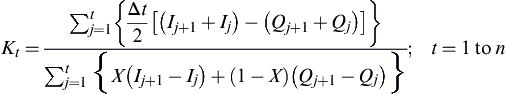
Approach I: The Muskingum method is a two-parameter linear model for channel routing. Parameters, K and X, of this method can be estimated from observed inflow and outflow hydrographs. Assuming the various values of X, and using the known values of the inflow and outflow hydrograph ordinates, the value of K can be determined as follows:

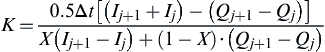$K = \frac{0.5 Δ t [(I_{j + 1} + I_{j}) - (Q_{j + 1} - Q_{j})]}{X (I_{j + 1} - I_{j}) + (1 - X) \cdot (Q_{j + 1} - Q_{j})}$ $K = \frac{0.5 Δ t [(I_{j + 1} + I_{j}) - (Q_{j + 1} - Q_{j})]}{X (I_{j + 1} - I_{j}) + (1 - X) \cdot (Q_{j + 1} - Q_{j})}$

(4.78)

The following steps are involved in determining parameters X and K.

1. In this procedure, the following equation derived from the continuity equation and the Muskingum-storage function is used, which is defined as follows:

$K_{t} = \frac{\sum_{j = 1}^{t} {\frac{Δ t}{2} [(I_{j + 1} + I_{j}) - (Q_{j + 1} + Q_{j})]}}{\sum_{j = 1}^{t} {X (I_{j + 1} - I_{j}) + (1 - X) (Q_{j + 1} - Q_{j})}}; t = 1 to n$ $K_{t} = \frac{\sum_{j = 1}^{t} {\frac{Δ t}{2} [(I_{j + 1} + I_{j}) - (Q_{j + 1} + Q_{j})]}}{\sum_{j = 1}^{t} {X (I_{j + 1} - I_{j}) + (1 - X) (Q_{j + 1} - Q_{j})}}; t = 1 to n$

(4.79)

where n is the number of observations.

2. The numerator and denominator of Eq. (4.79) are determined separately and plotted for each time interval on the vertical and horizontal axes, respectively. The plot derived usually forms a loop.

3. The value of X is considered appropriate which produces a loop close to a straight line.

4. The value of K is the slope of the straight line derived in Step 3.

Approach II: Another approach for estimating parameters K and X is as follows and is referred to as approach II. The steps involved are:

1. Determine the storage using the continuity equation defining the initial storage as follows:

$S_{j + 1} = S_{j} + Δ t [(I_{j + 1} + I_{j}) - (Q_{j + 1} + Q_{j})] / 2$ $S_{j + 1} = S_{j} + Δ t [(I_{j + 1} + I_{j}) - (Q_{j + 1} + Q_{j})] / 2$

(4.80)

2. Determine the Muskingum storage term with various values of X between 0 and 0.5. The storage function term is defined as follows:

$f_{j + 1} (X) = X I_{j + 1} + (1 - X) Q_{j + 1}$ $f_{j + 1} (X) = X I_{j + 1} + (1 - X) Q_{j + 1}$

(4.81)

3. The computed values of S_j+1 and f_i+1(X) are plotted for each time interval on the horizontal and vertical axes, respectively. The plots are usually a loop. The value of X that produces the loop close to a straight line is taken as the appropriate value.

4. The approximate straight line derived in Step 3 is used to determine parameter K. The value of K is determined as the slope of the straight line.

$K = \frac{S_{2} - S_{1}}{f_{1} - f_{2}}$ $K = \frac{S_{2} - S_{1}}{f_{1} - f_{2}}$

(4.82)

Approach III: The third approach for estimating the Muskingum parameters is based on the least-square method: The following equations are used in the least-square method:

$A = \frac{\sum_{j = 1}^{n} {Q_{j}}^{2} \cdot \sum_{j = 1}^{n} S_{j} I_{j} - \sum_{j = 1}^{n} Q_{j} I_{j} \cdot \sum_{j = 1}^{n} S_{j} Q_{j}}{\sum_{j = 1}^{n} {I_{j}}^{2} \cdot \sum_{j = 1}^{n} {Q_{j}}^{2} - {[\sum_{j = 1}^{n} Q_{j} I_{j}]}^{2}}$ $A = \frac{\sum_{j = 1}^{n} {Q_{j}}^{2} \cdot \sum_{j = 1}^{n} S_{j} I_{j} - \sum_{j = 1}^{n} Q_{j} I_{j} \cdot \sum_{j = 1}^{n} S_{j} Q_{j}}{\sum_{j = 1}^{n} {I_{j}}^{2} \cdot \sum_{j = 1}^{n} {Q_{j}}^{2} - {[\sum_{j = 1}^{n} Q_{j} I_{j}]}^{2}}$

(4.83)

$B = \frac{\sum_{j = 1}^{n} {I_{j}}^{2} \cdot \sum_{j = 1}^{n} S_{j} Q_{j} - \sum_{j = 1}^{n} Q_{j} I_{j} \cdot \sum_{j = 1}^{n} S_{j} I_{j}}{\sum_{j = 1}^{n} {I_{j}}^{2} \cdot \sum_{j = 1}^{n} {Q_{j}}^{2} - {[\sum_{j = 1}^{n} Q_{j} I_{j}]}^{2}}$ $B = \frac{\sum_{j = 1}^{n} {I_{j}}^{2} \cdot \sum_{j = 1}^{n} S_{j} Q_{j} - \sum_{j = 1}^{n} Q_{j} I_{j} \cdot \sum_{j = 1}^{n} S_{j} I_{j}}{\sum_{j = 1}^{n} {I_{j}}^{2} \cdot \sum_{j = 1}^{n} {Q_{j}}^{2} - {[\sum_{j = 1}^{n} Q_{j} I_{j}]}^{2}}$

(4.84)

$S_{j + 1} = S_{j} + Δ t [(I_{j + 1} + I_{j}) - (Q_{j + 1} + Q_{j})] / 2$ $S_{j + 1} = S_{j} + Δ t [(I_{j + 1} + I_{j}) - (Q_{j + 1} + Q_{j})] / 2$

(4.85)

$K = A + B$ $K = A + B$

(4.86)

$X = A / (A + B)$ $X = A / (A + B)$

(4.87)

Example 4.12:

Determine the outflow hydrograph using the Muskingum method for X = 0.15 and K = 2.30 h. The value of Q_t=1 h = 85 m³/s. The inflow hydrograph is given below:

Time (h)	1	2	3	4	5	6	7	8	9	10
I (m³/s)	93	137	208	320	442	546	630	678	691	675
Time (h)	11	12	13	14	15	16	17	18	19	20
I (m³/s)	634	571	477	390	329	247	184	134	108	90

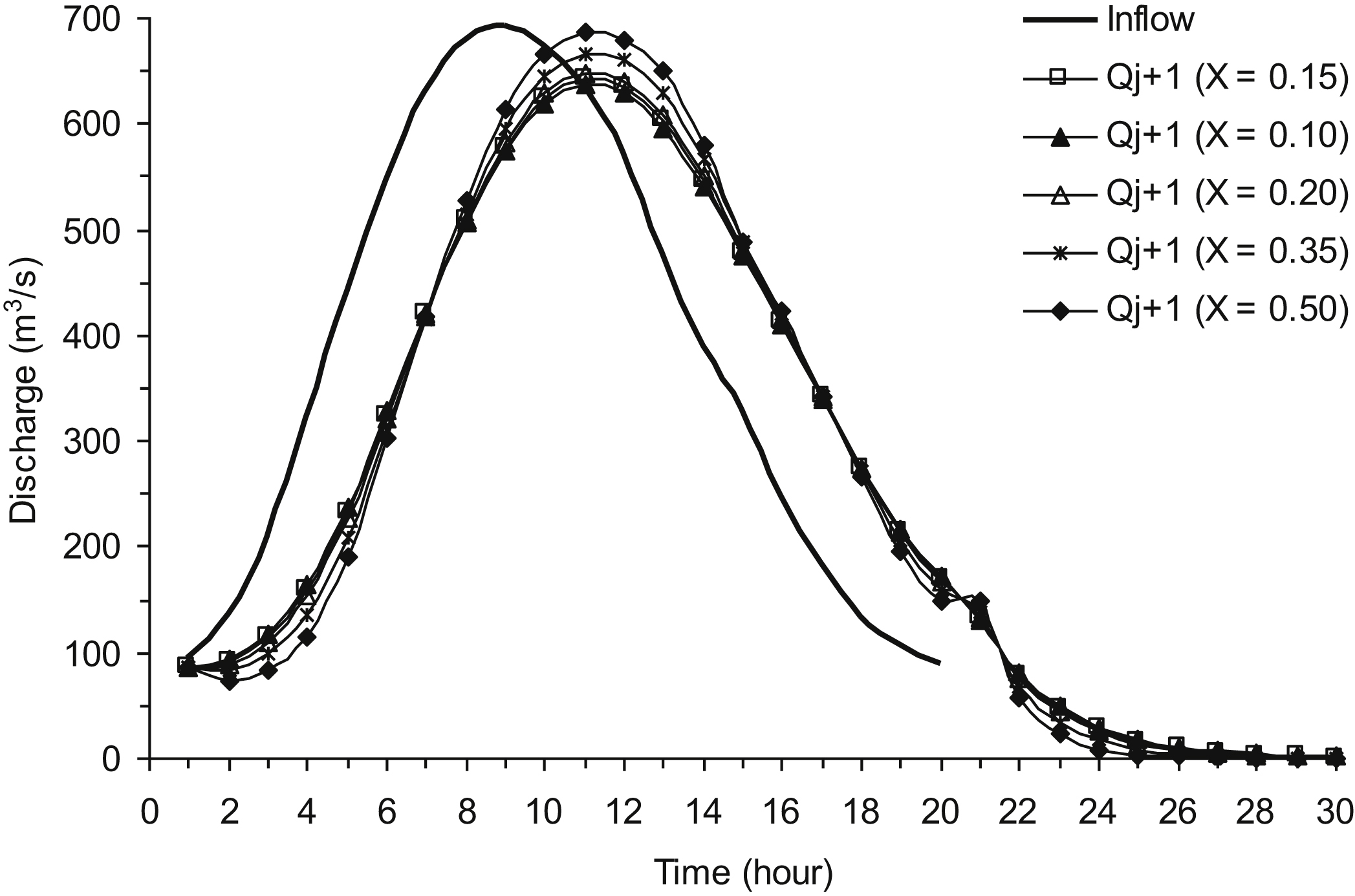
Also compare the shape of the outflow hydrograph for X = 0.10, 0.20, 0.35, and 0.50.

Solution:

Routing time interval, Δt = 1 h = 3600 s; X = 0.15; K = 2.30 h.

Using Eq. (4.74)–(4.77), Δt = 1 h, and K = 2.30 h, the routing coefficients of the Muskingum method are estimated. For various values of X, the coefficients are as follows:

Muskingum Routing Coefficients	X
Muskingum Routing Coefficients	0.15	0.10	0.20	0.35	0.50
$C_{1} = \frac{0.5 Δ t - K X}{0.5 Δ t + K (1 - X)}$ $C_{1} = \frac{0.5 Δ t - K X}{0.5 Δ t + K (1 - X)}$	0.0631	0.1051	0.0171	−0.1529	−0.3939
$C_{2} = \frac{0.5 Δ t + K X}{0.5 Δ t + K (1 - X)}$ $C_{2} = \frac{0.5 Δ t + K X}{0.5 Δ t + K (1 - X)}$	0.3442	0.2840	0.4103	0.6541	1.0000
$C_{3} = \frac{K (1 - X) - 0.5 Δ t}{0.5 Δ t + K (1 - X)}$ $C_{3} = \frac{K (1 - X) - 0.5 Δ t}{0.5 Δ t + K (1 - X)}$	0.5927	0.6109	0.5726	0.4987	0.3939
C₁ + C₂ + C₃	1.0000	1.0000	1.0000	1.0000	1.0000

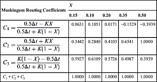
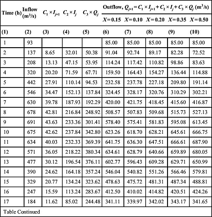
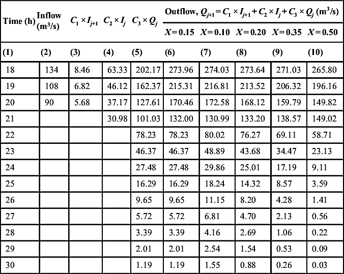
Using the estimated coefficients and the Muskingum routing equation (Eq. 4.73), the outflow hydrograph can be estimated. The computational steps are presented in Table 4.20.

The resulting outflow hydrographs for various values of X are shown in Fig. 4.9. Examining Fig. 4.9 gives the sensitivity of parameter X. For X = 0.5, there is no attenuation in the outflow hydrograph.

4.6.2.2. The Muskingum-Cunge Method

The Muskingum method accounts for the runoff diffusion by varying parameter X. The kinematic-wave approximation can produce a certain degree of numerical diffusion, depending upon the numerical approximation. In that case, the Muskingum and linear kinematic-wave routing equations are strikingly similar. However, the diffusion-wave approximation has the capacity to describe the physical diffusivity of the flood wave. Considering the aforesaid discussion, Cunge (1969) concluded that the Muskingum method is a linear kinematic-wave solution with numerical approximation which accounts for the numerical diffusion. To describe this, the kinematic-wave equation can be discretized in x–t plane in a way parallel to the Muskingum method. The discretization is based on centering the spatial derivative and off-centering the temporal derivative by means of a weighting factor X (Fig. 4.10) (Cunge, 1969; Ponce and Yevjevich, 1978; Singh, 1996).

Table 4.20

Determination of Outflow Hydrograph Using the Muskingum Method for Example 4.12

Time (h)	Inflow (m³/s)	C₁ × I_j+1	C₂ × I_j	C₃ × Q_j	Outflow, Q_j+1 = C₁ × I_j+1 + C₂ × I_j + C₃ × Q_j (m³/s)
Time (h)	Inflow (m³/s)	C₁ × I_j+1	C₂ × I_j	C₃ × Q_j	X = 0.15	X = 0.10	X = 0.20	X = 0.35	X = 0.50
(1)	(2)	(3)	(4)	(5)	(6)	(7)	(8)	(9)	(10)
1	93				85.00	85.00	85.00	85.00	85.00
2	137	8.65	32.01	50.38	91.04	92.74	89.17	82.28	72.52
3	208	13.13	47.15	53.95	114.24	117.42	110.82	98.86	83.63
4	320	20.20	71.59	67.71	159.50	164.43	154.27	136.44	114.88
5	442	27.91	110.14	94.53	232.58	237.78	227.18	209.80	191.14
6	546	34.47	152.13	137.84	324.45	328.17	320.76	310.29	302.21
7	630	39.78	187.93	192.29	420.00	421.75	418.45	415.60	416.87
8	678	42.81	216.84	248.92	508.57	507.83	509.68	515.73	527.13
9	691	43.63	233.36	301.41	578.40	575.41	581.83	595.08	613.45
10	675	42.62	237.84	342.80	623.26	618.70	628.21	645.61	666.75
11	634	40.03	232.33	369.39	641.75	636.30	647.51	666.61	687.90
12	571	36.05	218.22	380.34	634.61	628.79	640.66	659.89	680.05
13	477	30.12	196.54	376.11	602.77	596.43	609.28	629.71	650.99
14	390	24.62	164.18	357.24	546.04	540.82	551.26	566.46	579.81
15	329	20.77	134.24	323.62	478.63	475.72	481.31	487.34	488.81
16	247	15.59	113.24	283.67	412.50	410.02	414.82	420.51	424.26
17	184	11.62	85.02	244.48	341.11	339.97	342.02	343.17	341.65
Table Continued

Time (h)	Inflow (m³/s)	C₁ × I_j+1	C₂ × I_j	C₃ × Q_j	Outflow, Q_j+1 = C₁ × I_j+1 + C₂ × I_j + C₃ × Q_j (m³/s)
Time (h)	Inflow (m³/s)	C₁ × I_j+1	C₂ × I_j	C₃ × Q_j	X = 0.15	X = 0.10	X = 0.20	X = 0.35	X = 0.50
(1)	(2)	(3)	(4)	(5)	(6)	(7)	(8)	(9)	(10)
18	134	8.46	63.33	202.17	273.96	274.03	273.64	271.03	265.80
19	108	6.82	46.12	162.37	215.31	216.81	213.52	206.32	196.16
20	90	5.68	37.17	127.61	170.46	172.58	168.12	159.79	149.82
21			30.98	101.03	132.00	130.99	133.20	138.57	149.02
22				78.23	78.23	80.02	76.27	69.11	58.71
23				46.37	46.37	48.89	43.68	34.47	23.13
24				27.48	27.48	29.86	25.01	17.19	9.11
25				16.29	16.29	18.24	14.32	8.57	3.59
26				9.65	9.65	11.15	8.20	4.28	1.41
27				5.72	5.72	6.81	4.70	2.13	0.56
28				3.39	3.39	4.16	2.69	1.06	0.22
29				2.01	2.01	2.54	1.54	0.53	0.09
30				1.19	1.19	1.55	0.88	0.26	0.03

Figure 4.9 Inflow and outflow hydrograph for Example 4.12.

Discretizing the kinematic wave parallel to the Muskingum method,

$\frac{X (Q_{i}^{j + 1} - Q_{i}^{j}) + (1 - X) (Q_{i + 1}^{j + 1} - Q_{i + 1}^{j})}{Δ t} + c_{k} \frac{(Q_{i + 1}^{j} - Q_{i}^{j}) + (Q_{i + 1}^{j + 1} - Q_{i}^{j + 1})}{2 Δ x} = 0$ $\frac{X (Q_{i}^{j + 1} - Q_{i}^{j}) + (1 - X) (Q_{i + 1}^{j + 1} - Q_{i + 1}^{j})}{Δ t} + c_{k} \frac{(Q_{i + 1}^{j} - Q_{i}^{j}) + (Q_{i + 1}^{j + 1} - Q_{i}^{j + 1})}{2 Δ x} = 0$

(4.88)

where c_k = βV, a kinematic-wave celerity.

Solving Eq. (4.88) for

Q_{i + 1}^{j + 1}

$Q_{i + 1}^{j + 1}$

the result is:

$\frac{X}{Δ t} Q_{i}^{j + 1} - \frac{X}{Δ t} Q_{i}^{j} + \frac{(1 - X)}{Δ t} Q_{i + 1}^{j + 1} - \frac{(1 - X)}{Δ t} Q_{i + 1}^{j} + \frac{c_{k}}{2 Δ x} Q_{i + 1}^{j} - \frac{c_{k}}{2 Δ x} Q_{i}^{j} + \frac{c_{k}}{2 Δ x} Q_{i + 1}^{j + 1} - \frac{c_{k}}{2 Δ x} Q_{i}^{j + 1} = 0$ $\frac{X}{Δ t} Q_{i}^{j + 1} - \frac{X}{Δ t} Q_{i}^{j} + \frac{(1 - X)}{Δ t} Q_{i + 1}^{j + 1} - \frac{(1 - X)}{Δ t} Q_{i + 1}^{j} + \frac{c_{k}}{2 Δ x} Q_{i + 1}^{j} - \frac{c_{k}}{2 Δ x} Q_{i}^{j} + \frac{c_{k}}{2 Δ x} Q_{i + 1}^{j + 1} - \frac{c_{k}}{2 Δ x} Q_{i}^{j + 1} = 0$

$(\frac{(1 - X)}{Δ t} + \frac{c_{k}}{2 Δ x}) Q_{i + 1}^{j + 1} = (\frac{c_{k}}{2 Δ x} - \frac{X}{Δ t}) Q_{i}^{j + 1} + (\frac{c_{k}}{2 Δ x} + \frac{X}{Δ t}) Q_{i}^{j} + (\frac{(1 - X)}{Δ t} - \frac{c_{k}}{2 Δ x}) Q_{i + 1}^{j}$ $(\frac{(1 - X)}{Δ t} + \frac{c_{k}}{2 Δ x}) Q_{i + 1}^{j + 1} = (\frac{c_{k}}{2 Δ x} - \frac{X}{Δ t}) Q_{i}^{j + 1} + (\frac{c_{k}}{2 Δ x} + \frac{X}{Δ t}) Q_{i}^{j} + (\frac{(1 - X)}{Δ t} - \frac{c_{k}}{2 Δ x}) Q_{i + 1}^{j}$

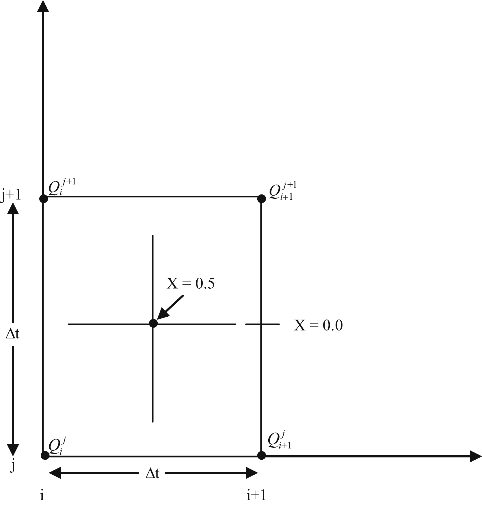
Figure 4.10 Discretization of kinematic-wave equation paralleling the Muskingum method (Ponce, 1989).

$\begin{matrix} \frac{2 (1 - X) + c_{k} (Δ t / Δ x)}{2 Δ x Δ t} \cdot Q_{i + 1}^{j + 1} = \frac{c_{k} (Δ t / Δ x) - 2 X}{2 Δ x Δ t} \cdot Q_{i}^{j + 1} + \frac{c_{k} (Δ t / Δ x) + 2 X}{2 Δ x Δ t} \cdot Q_{i}^{j} \\ + \frac{2 (1 - X) - c_{k} (Δ t / Δ x)}{2 Δ x Δ t} \cdot Q_{i + 1}^{j} \end{matrix}$ $\begin{matrix} \frac{2 (1 - X) + c_{k} (Δ t / Δ x)}{2 Δ x Δ t} \cdot Q_{i + 1}^{j + 1} = \frac{c_{k} (Δ t / Δ x) - 2 X}{2 Δ x Δ t} \cdot Q_{i}^{j + 1} + \frac{c_{k} (Δ t / Δ x) + 2 X}{2 Δ x Δ t} \cdot Q_{i}^{j} \\ + \frac{2 (1 - X) - c_{k} (Δ t / Δ x)}{2 Δ x Δ t} \cdot Q_{i + 1}^{j} \end{matrix}$

$\begin{matrix} Q_{i + 1}^{j + 1} = \frac{c_{k} (Δ t / Δ x) - 2 X}{2 (1 - X) + c_{k} (Δ t / Δ x)} \cdot Q_{i}^{j + 1} + \frac{c_{k} (Δ t / Δ x) - 2 X}{2 (1 - X) + c_{k} (Δ t / Δ x)} \cdot Q_{i}^{j} \\ + \frac{2 (1 - X) - c_{k} (Δ t / Δ x)}{2 (1 - X) + c_{k} (Δ t / Δ x)} \cdot Q_{i + 1}^{j} \end{matrix}$ $\begin{matrix} Q_{i + 1}^{j + 1} = \frac{c_{k} (Δ t / Δ x) - 2 X}{2 (1 - X) + c_{k} (Δ t / Δ x)} \cdot Q_{i}^{j + 1} + \frac{c_{k} (Δ t / Δ x) - 2 X}{2 (1 - X) + c_{k} (Δ t / Δ x)} \cdot Q_{i}^{j} \\ + \frac{2 (1 - X) - c_{k} (Δ t / Δ x)}{2 (1 - X) + c_{k} (Δ t / Δ x)} \cdot Q_{i + 1}^{j} \end{matrix}$

(4.89)

Eq. (4.89) can be written as follows:

$Q_{i + 1}^{j + 1} = C_{0} \cdot Q_{i}^{j + 1} + C_{1} \cdot Q_{i}^{j} + C_{2} \cdot Q_{i + 1}^{j}$ $Q_{i + 1}^{j + 1} = C_{0} \cdot Q_{i}^{j + 1} + C_{1} \cdot Q_{i}^{j} + C_{2} \cdot Q_{i + 1}^{j}$

(4.90)

$C_{0} = \frac{c_{k} (Δ t / Δ x) - 2 X}{2 (1 - X) + c_{k} (Δ t / Δ x)}$ $C_{0} = \frac{c_{k} (Δ t / Δ x) - 2 X}{2 (1 - X) + c_{k} (Δ t / Δ x)}$

(4.91)

$C_{1} = \frac{c_{k} (Δ t / Δ x) - 2 X}{2 (1 - X) + c_{k} (Δ t / Δ x)}$ $C_{1} = \frac{c_{k} (Δ t / Δ x) - 2 X}{2 (1 - X) + c_{k} (Δ t / Δ x)}$

(4.92)

$C_{2} = \frac{2 (1 - X) - c_{k} (Δ t / Δ x)}{2 (1 - X) + c_{k} (Δ t / Δ x)}$ $C_{2} = \frac{2 (1 - X) - c_{k} (Δ t / Δ x)}{2 (1 - X) + c_{k} (Δ t / Δ x)}$

(4.93)

Define:

$K = Δ x / c_{k}$ $K = Δ x / c_{k}$

(4.94)

Substitution of Eq. (4.94) into Eqs. (4.91)–(4.93) results in the routing coefficients of the Muskingum method. Therefore Eq. (4.94) confirms that K is the travel time of the flood wave, i.e., the time a given discharge takes to travel the reach length of Δx with the kinematic-wave celerity of c_k. In a linear model, c_k is constant and equal to the reference value; whereas it nonlinearly varies with the discharge.

In practice, the numerical diffusion can be used to simulate the physical diffusion of the actual flood wave. Expanding the discrete function Q(iΔx, jΔt) in Taylor series about the grid point (iΔx, jΔt), the numerical diffusion coefficient of the Muskingum scheme can be derived as follows (Ponce, 1989):

$D_{n} = c_{k} Δ x (\frac{1}{2} - X)$ $D_{n} = c_{k} Δ x (\frac{1}{2} - X)$

(4.95)

where D_n is the numerical diffusion coefficient of the Muskingum scheme. Eq. (4.95) reveals that:

1. for X = 0.5, the numerical diffusion will be zero, although there is numerical dispersion for c_k ≠ 1;

2. for X > 0.5, D_n < 0 which explains the behavior of the Muskingum method for this range of X values; and

3. for Δx = 0, D_n = 0, i.e., when space is zero the numerical diffusion will be zero.

Now, compare the numerical diffusivity (Eq. 4.95) with the hydraulic diffusivity which is given by:

$D_{h} = \frac{Q_{0}}{2 T S_{0}} = \frac{q_{0}}{2 S_{0}}$ $D_{h} = \frac{Q_{0}}{2 T S_{0}} = \frac{q_{0}}{2 S_{0}}$

(4.96)

The hydraulic diffusivity is a characteristic of flow and channel geometry, which is defined for the reference flow condition. In Eq. (4.96), q₀ = Q₀/T is the reference flow per unit channel width and D_h is the hydraulic diffusivity. From Eq. (4.96), it is observed that the hydraulic diffusivity is small for steep bottom slopes (for mountainous rivers), and large for mild bottom slopes for rivers in plain.

Comparing the numerical diffusivity with the hydraulic diffusivity, the result is:

$\frac{q_{0}}{2 S_{0}} = c_{k} Δ x (\frac{1}{2} - X)$ $\frac{q_{0}}{2 S_{0}} = c_{k} Δ x (\frac{1}{2} - X)$

(4.97)

Rearranging the terms of Eq. (4.97), the Muskingum weighting factor can be derived as:

$X = \frac{1}{2} (1 - \frac{q_{0}}{S_{0} c_{k} Δ x})$ $X = \frac{1}{2} (1 - \frac{q_{0}}{S_{0} c_{k} Δ x})$

(4.98)

With X calculated from Eq. (4.98), the Muskingum method becomes the Muskingum-Cunge method (NERC, 1975). Using Eq. (4.98), routing parameter X can be computed as a function of reach length Δx, reference discharge per unit width q₀, kinematic-wave celerity c_k, and bottom slope S₀.

To simulate the wave diffusion property with the Muskingum-Cunge method, it is necessary to optimize numerical diffusion (Eq. 4.98), while minimizing the numerical dispersion by keeping the value of Courant number C close to unity.

A unique feature of the Muskingum-Cunge method is the grid independence of the calculated outflow hydrograph, which sets it apart from other linear kinematic-wave solutions featuring uncontrolled numerical diffusion and dispersion by the convex method of kinematic-wave solution. If numerical dispersion in minimized, the calculated outflow at the downstream end of a channel reach will be essentially the same, regardless of how many subreaches are used in the computation. This is because X is a function of Δx, and routing coefficients C₀, C₁, and C₂ vary with reach length.

4.6.2.3. Modified Muskingum-Cunge Method (Ponce and Yevjevich, 1978)

An improved version of the Muskingum-Cunge method was given by Ponce and Yevjevich (1978). The modification of the Muskingum-Cunge method is based on incorporating the Courant number and cell Reynolds number. Courant number is defined as the ratio of wave celerity c_k to grid celerity Δx/Δt as follows:

$C = c_{k} \cdot \frac{Δ t}{Δ x}$ $C = c_{k} \cdot \frac{Δ t}{Δ x}$

(4.99)

The grid diffusivity is defined as the numerical diffusivity for X = 0. Therefore from Eq. (4.98), the grid diffusivity is defined as:

$D_{g} = \frac{c_{k} Δ x}{2}$ $D_{g} = \frac{c_{k} Δ x}{2}$

(4.100)

The cell Reynolds number (Roache, 1972) is defined as the ratio of hydraulic diffusivity (Eq. 4.96) to grid diffusivity (Eq. 4.100). This leads to

$D = \frac{D_{h}}{D_{g}} = \frac{q_{0} / 2 S_{0}}{c_{k} Δ x / 2} = \frac{q_{0}}{S_{0} c_{k} Δ x}$ $D = \frac{D_{h}}{D_{g}} = \frac{q_{0} / 2 S_{0}}{c_{k} Δ x / 2} = \frac{q_{0}}{S_{0} c_{k} Δ x}$

(4.101)

where D is the cell Reynolds number or the Peclet number. Therefore substituting the term D in Eq. (4.98) the result is:

$X = \frac{1}{2} (1 - D)$ $X = \frac{1}{2} (1 - D)$

(4.102)

Eqs. (4.99) and (4.102) imply that for very small value of Δx, D may be greater than 1, leading to negative values of X. In fact, for the characteristic reach length with D = 1, Eq. (4.101) gives the critical reach length as follows:

$Δ x_{c} = \frac{q_{0}}{S_{0} c_{k}}$ $Δ x_{c} = \frac{q_{0}}{S_{0} c_{k}}$

(4.103)

where Δx_c is the characteristic reach length (L). At D = 1, X = 0, i.e., routing gives only the translation effect. Therefore, in the Muskingum-Cunge method, the breach length shorter than Δx_c results in negative values of X. This should be contrasted with the classical Muskingum method, in which X is restricted between 0 and 0.5.

Substituting Eqs. (4.99) and (4.102) in Eqs. (4.91)–(4.93), the result is:

$C_{0} = \frac{- 1 + C + D}{1 + C + D}$ $C_{0} = \frac{- 1 + C + D}{1 + C + D}$

(4.104)

$C_{1} = \frac{1 + C - D}{1 + C + D}$ $C_{1} = \frac{1 + C - D}{1 + C + D}$

(4.105)

$C_{2} = \frac{1 - C + D}{1 + C + D}$ $C_{2} = \frac{1 - C + D}{1 + C + D}$

(4.106)

Routing coefficients (Eqs. 4.104–4.106) can be derived from the flow characteristics and channel geometry. Calculations can precede either linearly or nonlinearly. In a linear mode, routing parameters are estimated, based on the reference flow condition and kept constant throughout routing. For practical applications, either an average- or peak-flow value can be considered as a reference flow. Therefore the linear mode of computation is also referred to as the Constant Parameter Muskingum-Cunge method. When routing parameters vary with flow characteristics, it is referred to as the Variable Parameter Muskingum-Cunge method.

Example 4.13:

Use the constant parameter Muskingum-Cunge method to route the following inflow hydrograph.

Time (h)	0	1	2	3	4	5	6	7	8	9	10
Inflow (m³/s)	0	200	400	600	800	1000	800	600	400	200	0

The reference flow and channel characteristics are as follows:

Peak flow Q_P = 1000 m³/s, base flow Q_b = 0 m³/s, channel bottom slope S₀ = 0.000868, flow area at peak discharge A_P = 400 m², top width at peak discharge T_P = 100 m, rating exponent β = 1.6, reach length Δx = 14.4 km, and time interval Δt = 1 h.

Solution:

Using the given values, the peak discharge per unit width, q_p is determined:

$q_{p} = Q_{p} / T = 1000 / 100 = 10 m^{2} / s$ $q_{p} = Q_{p} / T = 1000 / 100 = 10 m^{2} / s$

Determine the velocity corresponding to the peak discharge, u:

$u = Q_{p} / A_{p} = 1000 / 400 = 2.5 m / s$ $u = Q_{p} / A_{p} = 1000 / 400 = 2.5 m / s$

Determine the kinematic-wave celerity c_k as follows:

$c_{k} = β u = 1.6 \times 2.5 = 4.0 m / s$ $c_{k} = β u = 1.6 \times 2.5 = 4.0 m / s$

Determine the advective Courant number C as follows (Eq. 4.99):

$C = c_{k} \cdot \frac{Δ t}{Δ x} = 4.0 \times \frac{3600}{14.4 \times 1000} = 1.0$ $C = c_{k} \cdot \frac{Δ t}{Δ x} = 4.0 \times \frac{3600}{14.4 \times 1000} = 1.0$

Determine the hydraulic diffusivity D_h for peak flow as follows (Eq. 4.96):

$D_{h} = \frac{q_{p}}{2 S_{0}} = \frac{10}{2 \times 0.000868} = 5760.37 m^{2} / s$ $D_{h} = \frac{q_{p}}{2 S_{0}} = \frac{10}{2 \times 0.000868} = 5760.37 m^{2} / s$

Determine the cell Reynolds number D as follows (Eq. 101):

$D = \frac{D_{h}}{D_{g}} = \frac{D_{h}}{c_{k} Δ x / 2} = \frac{5760.37}{4 \times (14.4 \times 1000) / 2} = 0.20$ $D = \frac{D_{h}}{D_{g}} = \frac{D_{h}}{c_{k} Δ x / 2} = \frac{5760.37}{4 \times (14.4 \times 1000) / 2} = 0.20$

Using the value of C and D, the routing coefficients of the Muskingum-Cunge method are estimated as follows (Eqs. 4.104–4.106):

$C_{0} = \frac{- 1 + C + D}{1 + C + D} = \frac{- 1 + 1 + 0.2}{1 + 1 + 0.2} = 0.0909$ $C_{0} = \frac{- 1 + C + D}{1 + C + D} = \frac{- 1 + 1 + 0.2}{1 + 1 + 0.2} = 0.0909$

$C_{1} = \frac{1 + C - D}{1 + C + D} = \frac{1 + 1 - 0.2}{1 + 1 + 0.2} = 0.8182$ $C_{1} = \frac{1 + C - D}{1 + C + D} = \frac{1 + 1 - 0.2}{1 + 1 + 0.2} = 0.8182$

$C_{2} = \frac{1 - C + D}{1 + C + D} = \frac{1 - 1 + 0.2}{1 + 1 + 0.2} = 0.0909$ $C_{2} = \frac{1 - C + D}{1 + C + D} = \frac{1 - 1 + 0.2}{1 + 1 + 0.2} = 0.0909$

$C_{1} + C_{2} + C_{3} = 0.0909 + 0.8182 + 0.0909 = 1.0$ $C_{1} + C_{2} + C_{3} = 0.0909 + 0.8182 + 0.0909 = 1.0$

Therefore the Muskingum-Cunge method becomes:

$Q_{i + 1}^{j + 1} = 0.0909 \times Q_{i}^{j + 1} + 0.8182 \times Q_{i}^{j} + 0.0909 \times Q_{i + 1}^{j}$ $Q_{i + 1}^{j + 1} = 0.0909 \times Q_{i}^{j + 1} + 0.8182 \times Q_{i}^{j} + 0.0909 \times Q_{i + 1}^{j}$

Computations are given in Table 4.21. Comparison of inflow and routed hydrographs is shown in Fig. 4.11.

..................Content has been hidden....................

You can't read the all page of ebook, please click here login for view all page.

Table of Contents for 4.6. Inflow Estimation in Multi-Reservoir Case

Create new playlist

Sign In

Sign Up

4.6. Inflow Estimation in Multi-Reservoir Case

4.6.1. Reservoir Routing: Storage-Indication Method

4.6.2. Channel Routing

4.6.2.1. The Muskingum Method

4.6.2.1.1. Parameter Estimation of the Muskingum Method

4.6.2.2. The Muskingum-Cunge Method

4.6.2.3. Modified Muskingum-Cunge Method (Ponce and Yevjevich, 1978)

Table of Contents for
4.6. Inflow Estimation in Multi-Reservoir Case