Search in book...
Toggle Font Controls
Create new playlist

Name your new playlist

Playlist description (optional)
Sign In

Email address

Password

Forgot Password?

or

Continue with Facebook

Continue with Google
Sign Up

Full Name

Email address

Confirm Email Address

Password

or

Continue with Facebook

Continue with Google

Chapter 12

Irrigation Scheduling

Abstract

For effective management and to improve the productivity of irrigation water, both temporal and spatial distribution of irrigation supply are important. The timely irrigation supply with desirable quantity is dealt with by irrigation scheduling, whereas the equitable distribution of irrigation supply can be met through the Warabandi scheduling. In this chapter, both the aspects are suitably covered. For irrigation scheduling, two methods are described, one based on simple calculation and the other based on the water balance approach. The former method gives a general idea of the irrigation interval, whereas the latter method gives detailed soil moisture accounting in the field and is more robust than the former method. The water balance method can be used for real-time irrigation scheduling and can be linked to the climatic forecast to assess the agricultural drought. In the second part of the chapter, the Warabandi scheduling is discussed.

Keywords

Irrigation scheduling; Real-time irrigation; Soil moisture balance; Spatial distribution; Temporal distribution; Warabandi scheduling; Water balance

For effective management and improvement of the productivity of irrigation water, both temporal and spatial distribution of irrigation supply are important. Timely irrigation supply with desirable quantity is dealt with by irrigation scheduling, whereas the equitable distribution of irrigation supply can be met through the Warabandi scheduling. In this chapter both the aspects will be discussed. First, irrigation scheduling will be discussed in detail, followed by Warabandi scheduling.

Irrigation scheduling can be defined as “the process of determining when to irrigate and how much water to apply, based upon measurements or estimates of soil water or water used by the plant” (ASABE, 2007). The method of estimating irrigation scheduling depends on either soil or plant monitoring or soil water balance estimates. Methods for monitoring or estimating the soil water status or evapotranspiration (ET) include the hand feel and appearance of soil, gravimetric soil water sampling, tensiometers, electrical resistance blocks, water balance approaches, and modified atmometer (Broner, 2005). Here, two methods are described for irrigation scheduling: simple calculation method (FAO, 1989) and water balance approach. The former method gives a general idea of the irrigation interval (INT) and accounts for the climatic parameters, and, therefore, is considered good. The latter method gives detailed soil moisture accounting in the field and is more robust than the former method. The water balance method can be used for real-time irrigation scheduling and can include the climatic forecast.

12.1. Simple Calculation of Irrigation Scheduling (FAO, 1989)

The simple calculation method to determine the irrigation schedule is based on the estimated depth of irrigation application and the calculated irrigation water need (IN) of the crop over the growing season. The following steps are involved in the estimation of the irrigation schedule (FAO, 1989):

1. Estimate the net and gross irrigation depth (d_net and d_gross), in millimeters;

2. Estimate the IN in millimeter over the total growing season;

3. Estimate the number of irrigation applications over the total growing season;

4. Estimate the INT, in days; and

5. Adjust for the peak irrigation demand.

Step 1: Estimation of the net and gross irrigation depth

The net irrigation depth is best determined locally by checking how much water is given per irrigation application with the local irrigation method and practice. In the absence of local irrigation application data, Table 12.1 can be used to estimate the net irrigation depth with the aid of Table 12.2, which summarizes the approximate rooting depth (RD) of major crops.

Table 12.1

Approximate Net Irrigation Depth Applied per Irrigation (mm) (FAO, 1989)

Soil Type	Shallow Rooting Depth Crops	Medium Rooting Depth Crops	Deep Rooting Depth Crops
Shallow and/or sandy soil	15	30	40
Loamy soil	20	40	60
Clayey soil	30	50	70

Table 12.2

Approximate Root Depth of the Major Crops (FAO, 1989)

Depth Class/Rooting Depth Range	Crops
Shallow rooting crops (30–60 cm)	Crucifers (cabbage, cauliflower, etc.), celery, lettuce, onions, pineapple, potatoes, spinach, other vegetables except beat, carrot, cucumber
Medium rooting crops (50–100 cm)	Banana, beans, beat, carrot, clover, cucumber, groundnut, palm trees, peas, pepper, sisal, soybeans, sugar beet, sunflower, tobacco, tomatoes
Deep rooting crops (90–150 cm)	Alfalfa, barley, citrus, cotton, deciduous orchards, flax, grapes, maize, melons, oats, olives, safflower, sorghum, sugarcane, sweet potatoes, wheat

The gross irrigation depth can be estimated using the following expression:

$d_{g r o s s} = \frac{d_{n e t}}{E_{a}} \times 100$ $d_{g r o s s} = \frac{d_{n e t}}{E_{a}} \times 100$

(12.1)

where d_gross is the gross irrigation depth (mm) and E_a is the field application efficiency (%). Typical values of the field application efficiency are given in Table 12.3.

Step 2: Estimation of IN

The procedure for estimation of irrigation water requirement has been discussed in detail earlier. For the growing period, if the percolation loss and ground water contribution from the field are considered negligible then the IN can be estimated as follows:

${IN}_{i} = E T_{c, i} - P_{e, i}$ ${IN}_{i} = E T_{c, i} - P_{e, i}$

(12.2)

where ET_c,i is the crop water demand for the ith growing period (mm) and P_e,i is the effective rainfall during the ith period (mm). The total net IN during the total growing period is estimated as:

Table 12.3

Typical Values of Field Application Efficiency, E_a (FAO, 1989)

S. No.	Irrigation Method	E_a (%)
1	Surface irrigation	60
2	Sprinkler irrigation	75
3	Drip irrigation	90

$IN = \sum_{i = 1}^{N D_{c}} {IN}_{i}$ $IN = \sum_{i = 1}^{N D_{c}} {IN}_{i}$

(12.3)

where ND_c is the total growing period. If detailed climatic data are not available, the approximate value of crop water needs, ET_c, can be determined from Table 12.4.

Step 3: Estimation of the number of irrigation applications over the total growing season

The number of irrigation applications over the total growing season can be obtained as follows:

$Number of Irrigation (N_{I}) = \frac{IN}{d_{n e t}}$ $Number of Irrigation (N_{I}) = \frac{IN}{d_{n e t}}$

(12.4)

Table 12.4

Crop Water Need and Growing Period (FAO, 1989)

Crop	Crop Water Need, ET_c (mm)	Crop Growing Period, N_c (days)
Alfalfa	800–1600	100–365
Banana	1200–2200	300–365
Barley/wheat/oats	450–650	120–150
Bean (green)	300–500	75–90
Cabbage	350–500	120–140
Citrus	900–1200	240–365
Cotton	700–1300	180–195
Maize	500–800	125–180
Melon	400–600	120–160
Onion	350–550	150–210
Peanut/Groundnut	500–700	130–140
Pea	350–500	90–100
Pepper	600–900	120–210
Potato	500–700	105–145
Paddy	450–700	90–150
Sorghum	450–650	120–130
Soybean	450–700	130–150
Sugar beat	550–750	160–230
Sugarcane	1500–2500	270–365
Sunflower	600–1000	125–130
Tomato	400–800	135–180

Step 4: Estimation of the INT

The INT can be estimated as follows:

$INT = \frac{N D_{c}}{N_{I}}$ $INT = \frac{N D_{c}}{N_{I}}$

(12.5)

where INT is calculated in days, ND_c is the total growing period of the crop (days), and N_I is the number of irrigation.

Step 5: Adjustment for peak period

For peak period, the irrigation need for the crop is less than the net irrigation depth, therefore, steps 2 and 4 are repeated for the peak period adjustment. Considering the aforementioned algorithm of simple irrigation scheduling method, software can be developed on Microsoft Office-Excel platform. A sample computation of irrigation scheduling using the previously described method is presented in Example 12.1.

Example 12.1:

For the groundnut crop, the following information is collected from the field.

Soil type: loam

Irrigation method: furrow

Field application efficiency, E_a = 60%

Total crop growing period, ND_c = 130 days

Planting date: 15th July

Harvesting date: 25th November

The IN during the growing period is as follows:

Month	Jul.	Aug.	Sep.	Oct.	Nov.	Total
IN (mm/month)	38	115	159	170	45	527

Using this information the irrigation schedule is determined for: (1) total growing period, (2) peak period, and (3) the combination of (1) and (2).

Solution:

Using the software, the computations are as follows:

(A) Project and watercourse
Project	Ex. 12.1
Outlet no.	Ex. 12.1
Location: Latitude		Longitude	Altitude(m)
Culturable command area (CCA)
Irrigated command area (ICA)
Outlet capacity (cumec)
(B) CCA, soil and area under cultivation
ICA (ha)
Table Continued

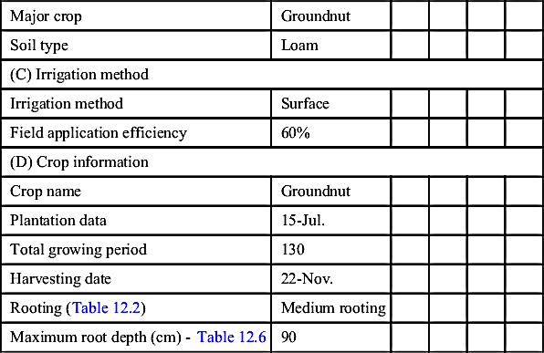
Major crop	Groundnut
Soil type	Loam
(C) Irrigation method
Irrigation method	Surface
Field application efficiency	60%
(D) Crop information
Crop name	Groundnut
Plantation data	15-Jul.
Total growing period	130
Harvesting date	22-Nov.
Rooting (Table 12.2)	Medium rooting
Maximum root depth (cm) - Table 12.6	90

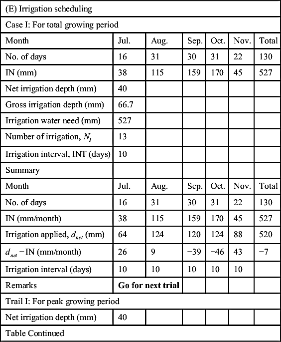
(E) Irrigation scheduling
Case I: For total growing period
Month	Jul.	Aug.	Sep.	Oct.	Nov.	Total
No. of days	16	31	30	31	22	130
IN (mm)	38	115	159	170	45	527
Net irrigation depth (mm)	40
Gross irrigation depth (mm)	66.7
Irrigation water need (mm)	527
Number of irrigation, N_I	13
Irrigation interval, INT (days)	10
Summary
Month	Jul.	Aug.	Sep.	Oct.	Nov.	Total
No. of days	16	31	30	31	22	130
IN (mm/month)	38	115	159	170	45	527
Irrigation applied, d_net (mm)	64	124	120	124	88	520
d_net − IN (mm/month)	26	9	−39	−46	43	−7
Irrigation interval (days)	10	10	10	10	10
Remarks	Go for next trial
Trail I: For peak growing period
Net irrigation depth (mm)	40
Table Continued

Gross irrigation depth (mm)	66.7
IN during peak period (mm)	329
Number of days during peak	61
Number of irrigation, N_I	8.5
Irrigation interval, INT (days)	7
Summary
Month	Jul.	Aug.	Sep.	Oct.	Nov.	Total
No. of days	16	31	30	31	22	130
IN (mm/month)	38.00	115.00	159.00	170.00	45.00	527.00
Irrigation applied, d_net (mm)	64.00	124.00	171.43	177.14	88.00	624.57
d_net − IN (mm/month)	26.00	9.00	12.43	7.14	43.00	97.57
Irrigation interval	10	10	7	7	10
Remarks	Irrigation scheduling completed

12.2. Water Balance Method

The water balance is the accounting procedure of all inflows, outflows, and storages involved within the firm hydrologic boundary during a given period of time. For irrigated fields, the farm land will act as a hydrologic boundary and the lower boundary is up to the RD. The water balance is merely a detailed statement of the law of conservation of mass. The water balance can be expressed as follows:

$Inflows - Outflows = Change in Storages$ $Inflows - Outflows = Change in Storages$

(12.6)

Mathematically, a general water balance or soil moisture balance equation can be expressed as follows:

${(P + I + U)}_{j + 1} - {(Q + D + \bar{E} {\bar{T}}_{c})}_{j + 1} = Δ {SM}_{j}$ ${(P + I + U)}_{j + 1} - {(Q + D + \bar{E} {\bar{T}}_{c})}_{j + 1} = Δ {SM}_{j}$

(12.7)

Substituting ΔSM_j = SM_j+1 − SM_j in Eq. (12.7) results:

${SM}_{j + 1} = {SM}_{j} + {(P - Q - D)}_{j + 1} + {(I + U)}_{j + 1} - E T_{c, j}$ ${SM}_{j + 1} = {SM}_{j} + {(P - Q - D)}_{j + 1} + {(I + U)}_{j + 1} - E T_{c, j}$

(12.8)

${SM}_{j + 1} = {SM}_{j} + R e_{j + 1} + (I_{j + 1} + U_{j + 1}) - E T_{c, j}$ ${SM}_{j + 1} = {SM}_{j} + R e_{j + 1} + (I_{j + 1} + U_{j + 1}) - E T_{c, j}$

(12.9)

Converting Eq. (12.9) into a soil moisture deficit (SWD_j = FC − SM_j) term will result in:

${SWD}_{j + 1} = {SWD}_{j} + {({\bar{E} \bar{T}}_{c} - I - U)}_{j + 1} - {(R_{e})}_{j + 1}$ ${SWD}_{j + 1} = {SWD}_{j} + {({\bar{E} \bar{T}}_{c} - I - U)}_{j + 1} - {(R_{e})}_{j + 1}$

(12.10)

In this governing equation, P is the precipitation or rainfall, I is the irrigation water applied, U is the upward flux of water to the root zone depth or capillary rise, Q is the surface runoff from the field, D is the deep percolation, ET_c is the average evapotranspiration from the cropped surface or consumptive use of crop during the water balance period, ΔSM is the change in soil moisture storage, SM_j is the soil moisture at the jth time, SM_j + 1 is the soil moisture at the (j + 1)th time step, SWD is the soil moisture deficit, FC is the field capacity of soil, and R_e is the effective rainfall that replenishes the soil, while rainfall or precipitation occurs. All the terms appearing in the previous equation are either in volumetric unit or in water depth equivalent unit. For irrigation scheduling, daily time steps are common and users are most often interested in estimating the irrigation amount(s) and date(s) of application needed to maintain the soil water deficit (SWD) at some future date at or above the maximum/management allowable deficit or depletion (MAD).

12.2.1. Soil Moisture Terminology

A description of the soil moisture terms appearing in Eqs. (12.8)–(12.10) is presented as follows:

1. FC: The term field capacity is interchangeably used with the terms water holding capacity and water retention capacity. FC is the amount of soil moisture or water content held in soil after excess water has drained away and the rate of downward movement has materially decreased, which usually takes place within 2–3 days after a rain or irrigation in pervious soils of uniform structure and texture. The physical definition of FC (θ_FC) is the bulk water content retained in soil at −33 J/kg (or −0.33 bar) of hydraulic head or suction pressure. In equivalent depth, it is:

$FC = (θ_{FC} / 100) \times RD$ $FC = (θ_{FC} / 100) \times RD$

(12.11)

where FC is the field capacity (mm), θ_FC is the field capacity of soil (%v/v), and RD is the rooting depth (mm).

2. Permanent wilting point (PWP): It is the point when there is no water available to the plant. PWP depends on the plant variety, but it is usually around 1500 kPa (15 bars). At this stage, the soil still contains some water, but it is difficult for the roots to extract from the soil. It is also presented in percentage by volume (%v/v) and can be converted into the depth term by multiplying with root depth (RD) as explained in Eq. (12.11).

3. Available water content: It is the amount of water actually available to the plants for their growth. It is determined as FC minus the water that will remain in the soil at PWP. The available water content depends greatly on the soil texture and structure.

The moisture at the available water capacity is expressed as follows:

$θ_{AWC} = θ_{FC} - θ_{PWP}$ $θ_{AWC} = θ_{FC} - θ_{PWP}$

(12.12)

where θ_AWC is the maximum available moisture content (%v/v), θ_FC is the moisture content at the FC (%v/v), and θ_PWP is the moisture content at the PWP (%v/v). The values of θ_FC, θ_PWP, and available water holding capacity (AWC) are summarized in Table 12.5 for various soil textures.

4. AWC: The available water content (cm/cm) is determined as follows:

$AWC = \frac{θ_{FC} - θ_{PWP}}{100}$ $AWC = \frac{θ_{FC} - θ_{PWP}}{100}$

(12.13)

The total water available in the root zone (TAW) is determined as:

$TAW = AWC \times RD = \frac{θ_{FC} - θ_{PWP}}{100} \times RD$ $TAW = AWC \times RD = \frac{θ_{FC} - θ_{PWP}}{100} \times RD$

(12.14)

Table 12.5

Soil moisture at field capacity (θ_FC), permanent wilting point (θ_PWP), available water content (AWC in cm/cm), and basic infiltration rate (F in mm/day)

Soil Type	θ_FC (%v)	θ_PWP (%v)	F (mm/day)	AWC (cm/cm)
Sand	9.0	4.0	1,200	0.050
	(6–12)	(2–6)	(600–6,000)
Coarse sand	3.2	1.2	11,200	0.020
Medium coarse sand	9.5	1.7	3,000	0.078
Medium fine sand	15.5	2.3	1,100	0.132
Fine sand	19.6	4.2	500	0.154
Sandy loam	14.0	6.0	600	0.080
	(10–18)	(4–8)	(312–1,824)
Sandy loam	19.5	6.1	165	0.134
Light loamy medium (coarse sand)	24.2	10.0	23	0.142
Loamy medium coarse sand	18.1	2.1	3.6	0.160
Loamy fine sand	14.6	6.0	265	0.086
Fine sandy loam	27.3	8.7	120	0.186
Loam	22.0	13.0	192	0.090
	(18–26)	(8–12)	(192–480)
Silt loam	33.8	9.2	6.5	0.246
Loam	29.3	9.8	50	0.195
Clay loam	27.0	13.0	192	0.140
	(23–31)	(11–15)	(60–360)
Sandy clay loam	31.7	18.0	235	0.137
Silty clay loam	34.5	18.5	15	0.160
Clay loam	39.3	25.5	9.8	0.138
Silt clay	31.0	15.0	60	0.160
	(27–35)	(13–17)	(7.2–120)
Clay	35.0	17.0	12	0.180
	(31–39)	(15–19)	(2.4–120)
Light clay	34.0	21.5	35	0.125
Silty clay	44.7	25.7	13	0.190
Basin clay	49.8	32.1	2.2	0.177

5. Currently available soil moisture (SM): It is defined as the moisture currently (i.e., at the present state of crop and soil) available to plants. Mathematically, it is expressed as follows:

$θ_{SM} = θ_{0} - θ_{PWP}$ $θ_{SM} = θ_{0} - θ_{PWP}$

(12.15)

where θ_SM is the currently available soil moisture content (%v/v) and θ₀ is the current soil moisture content (%v/v). It can be presented in the depth term through the following equation:

$SM = \frac{θ_{0} - θ_{PWP}}{100} \times RD$ $SM = \frac{θ_{0} - θ_{PWP}}{100} \times RD$

(12.16)

6. Depletion of available soil moisture: The percentage depletion of available soil water is the lowering of current state of soil moisture from FC with respect to the theoretical maximum possible available soil moisture. It is expressed as follows:

$Depletion, % = \frac{θ_{FC} - θ_{0}}{θ_{FC} - θ_{PWP}} \times 100$ $Depletion, % = \frac{θ_{FC} - θ_{0}}{θ_{FC} - θ_{PWP}} \times 100$

(12.17)

7. SWD: It is the difference between FC (θ_FC) and current soil moisture content (θ_j) and can be determined as follows:

${SWD}_{j} = θ_{FC} - θ_{j}$ ${SWD}_{j} = θ_{FC} - θ_{j}$

(12.18)

In the volumetric depth term, the soil moisture deficit (mm/mm) is given by the following formula:

${SWD}_{j} = FC - {SM}_{j}$ ${SWD}_{j} = FC - {SM}_{j}$

(12.18a)

8. MAD: In irrigation practice, only a percentage of AWC is allowed to be depleted, because plants start to experience water stress even before soil water is depleted down to PWP. Therefore MAD (%) of the AWC must be specified while scheduling irrigation. Therefore MAD is the fraction/percentage of total plant available water that is to be depleted from the active root zone before irrigation is applied. This amount is managed by the water manager and depends on the soil texture and type of crop.

The MAD can be expressed in terms of depth of water (d_MAD, mm) using the following equation.

$d_{MAD} = (MAD / 100) \times AWC \times RD = (MAD / 100) \times TAW$ $d_{MAD} = (MAD / 100) \times AWC \times RD = (MAD / 100) \times TAW$

(12.19)

The value of d_MAD can be used as a guide for deciding when to irrigate. Typically, irrigation water should be applied when SWD → d_MAD or when SWD ≥ d_MAD. To minimize the water stress on the crop, SWD should be kept less than d_MAD (i.e., SWD < d_MAD) if irrigation system has enough capacity. The net irrigation amount equal to SWD can be applied to bring soil moisture deficit to zero or at FC. If the irrigation system has limited capacity (maximum irrigation amount is less than d_MAD), then the irrigator should not wait for SWD → d_MAD, but should irrigate more frequently to ensure SWD < d_MAD.

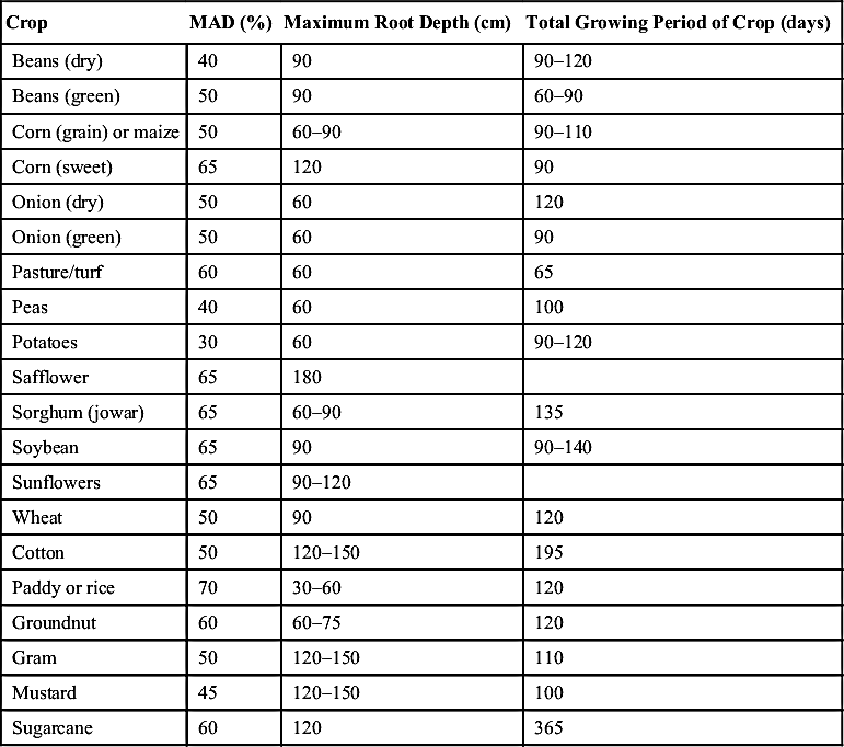
The MAD and maximum rooting depth of selected crops are summarized in Table 12.6.

Table 12.6

Maximum/management Allowable Depletion (MAD) and Rooting Depth for Crops (FAO, 1989)

Crop	MAD (%)	Maximum Root Depth (cm)	Total Growing Period of Crop (days)
Beans (dry)	40	90	90–120
Beans (green)	50	90	60–90
Corn (grain) or maize	50	60–90	90–110
Corn (sweet)	65	120	90
Onion (dry)	50	60	120
Onion (green)	50	60	90
Pasture/turf	60	60	65
Peas	40	60	100
Potatoes	30	60	90–120
Safflower	65	180
Sorghum (jowar)	65	60–90	135
Soybean	65	90	90–140
Sunflowers	65	90–120
Wheat	50	90	120
Cotton	50	120–150	195
Paddy or rice	70	30–60	120
Groundnut	60	60–75	120
Gram	50	120–150	110
Mustard	45	120–150	100
Sugarcane	60	120	365

12.2.2. Rooting Depth

During the progression of crop development, the variation in the root zone depth for the crop can be determined using the following formula proposed by Borg and Grimes (1986):

${RD}_{j + 1} = {RD}_{\max} [0.5 + 0.5 \times \sin {3.03 \times (DAP / DTM) - 1.47}]$ ${RD}_{j + 1} = {RD}_{\max} [0.5 + 0.5 \times \sin {3.03 \times (DAP / DTM) - 1.47}]$

(12.20)

RD_j + 1 ≥ 150 mm (As evapotranspiration takes place up to 150 mm of soil depth).

In Eq. (12.20), DAP is the duration in days after planting, i.e., ( j + 1)th day; DTM is the days at which the maximum RD is attained by crop, i.e., RD_max; RD_j + 1 is the RD in mm on ( j + 1)th day; and RD_max is the maximum RD in mm on DTM. The values of RD_max and DTM is given in Table 12.6.

12.2.3. Estimation of Crop Evapotranspiration (ET_c)

The crop evapotranspiration (ET_c) is estimated using the following formula:

$E T_{c} = E T_{o} \times K_{c} \times K_{s}$ $E T_{c} = E T_{o} \times K_{c} \times K_{s}$

(12.21)

where ET_c is the crop evapotranspiration or consumptive use (mm), ET_o is the reference crop evapotranspiration (mm), K_c is the crop coefficient, and K_s is the water stress coefficient. A typical curve for K_c used in the computation of irrigation scheduling with daily time step is shown in Fig. 12.1. A detailed procedure for estimating ET_c is given in Chapters 5 and 6, in which the value of ET_o is estimated using the Penman–Monteith method when climatic data, such as temperature, wind speed, relative humidity, and sunshine hours, are available. Under limited climatic data, the Hargreaves method (Hargreaves and Samani, 1985; Hargreaves, 1994) can be satisfactorily used and is expressed as follows. The Hargreaves equation has a tendency to underpredict under high-wind-speed conditions (u > 3 m/s) and overpredict under conditions of high relative humidity.

$E T_{o} = 0.0023 (T_{mean} + 17.8) {(T_{\max} - T_{\min})}^{0.5} \times (0.408 \times R_{a})$ $E T_{o} = 0.0023 (T_{mean} + 17.8) {(T_{\max} - T_{\min})}^{0.5} \times (0.408 \times R_{a})$

(12.22)

where ET_o is the reference evapotranspiration (mm/d); T_mean, T_max, and T_min are the daily mean, maximum, and minimum temperatures (°C), respectively; and R_a is the extraterrestrial radiation for each day (MJ/m² d). A detailed procedure for estimating the value of R_a is summarized in Chapter 5.

Figure 12.1 Generalized crop coefficient curves (FAO, 1998).

The values of crop coefficient for selected crops are also summarized in Chapter 5. The value of water stress coefficient, K_s, varies between 0 and 1 and depends on the SWD. If SWD remains less than d_MAD, K_s = 1, which means no water stress condition. Otherwise, it would be less than unity. The value of K_s can be determined using the following relationship:

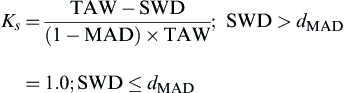$\begin{matrix} K_{s} = \frac{TAW - SWD}{(1 - MAD) \times TAW}; SWD > d_{MAD} \\ = 1.0; SWD \leq d_{MAD} \end{matrix}$ $\begin{matrix} K_{s} = \frac{TAW - SWD}{(1 - MAD) \times TAW}; SWD > d_{MAD} \\ = 1.0; SWD \leq d_{MAD} \end{matrix}$

(12.23)

12.2.4. Estimation of Effective Rainfall

To estimate the irrigation water requirement, it is required to know the portion of rainfall useful to the crop root zone. Not all rainfall infiltrates into the soil; a part may evaporate; another part may become surface runoff. Therefore the effective rainfall is that part of the total precipitation that replaces, or potentially reduces, a corresponding net quantity of the required irrigation water. Based on the ICID (1978), the definition of effective rainfall can be given as: “effective rainfall or precipitation is that part of the total precipitation on the cropped area, during a specific time period, which is available to meet the potential transpiration requirements in the cropped area.”

In irrigation scheduling algorithm, the SCS-CN method has been used and is discussed below.

12.2.4.1. The SCS-CN Method

The SCS-CN method is based on the water balance equation and two fundamental hypotheses. The first hypothesis equates the ratio of the actual amount of direct surface runoff (Q) to the total rainfall (P) (or maximum potential surface runoff) to the ratio of the amount of actual infiltration (F) to the amount of the potential maximum retention (S). The second hypothesis relates the initial abstraction (I_a) to the potential maximum retention. Thus the SCS-CN method consists of:

1. Water balance equation (USDA, 1972; McCuen, 1982; Mishra and Singh, 2003):

$P = I_{a} + F + Q$ $P = I_{a} + F + Q$

(12.24)

$P = R_{e} + Q$ $P = R_{e} + Q$

(12.25)

where R_e is the effective rainfall represented by:

$R_{e} = I_{a} + F$ $R_{e} = I_{a} + F$

(12.26)

$R_{e} = I_{a} + F = P - Q$ $R_{e} = I_{a} + F = P - Q$

(12.27)

2. Proportional equality hypothesis:

$\frac{Q}{P - I_{a}} = \frac{F}{S}$ $\frac{Q}{P - I_{a}} = \frac{F}{S}$

(12.28)

3. I_a-S hypothesis:

$I_{a} = λ S$ $I_{a} = λ S$

(12.29)

where P is the total rainfall, I_a is the initial abstraction, F is the cumulative infiltration excluding I_a, Q is the direct runoff, and S is the potential maximum retention or infiltration, also described as the potential initial abstraction retention (McCuen, 2002). All quantities in Eqs. (12.24)–(12.29) are in depth or volumetric units. For irrigation purposes, the term F + I_a in Eqs. (12.26) and (12.27) equals the effective rainfall, R_e (i.e., R_e = P − Q).

Combining Eqs. (12.24) and (12.28) results in the following expression:

$\begin{matrix} Q = \frac{{(P - I_{a})}^{2}}{P - I_{a} + S}; for P \geq I_{a} \\ Q = 0; for P < I_{a} \end{matrix}$ $\begin{matrix} Q = \frac{{(P - I_{a})}^{2}}{P - I_{a} + S}; for P \geq I_{a} \\ Q = 0; for P < I_{a} \end{matrix}$

(12.30)

For λ = 0.2, Eq. (12.30) can be rewritten as

$\begin{matrix} Q = \frac{{(P - 0.2 S)}^{2}}{P + 0.8 S}; for P \geq 0.2 S \\ Q = 0; for P < 0.2 S \end{matrix}$ $\begin{matrix} Q = \frac{{(P - 0.2 S)}^{2}}{P + 0.8 S}; for P \geq 0.2 S \\ Q = 0; for P < 0.2 S \end{matrix}$

(12.31)

Since parameter S (Eqs. 12.30 and 12.31) can vary in the range of 0 ≤ S ≤ ∞, it is mapped into a dimensionless curve number (CN), varying in a more appealing range 0 ≤ CN ≤ 100, as follows:

$S = \frac{25400}{CN} - 254$ $S = \frac{25400}{CN} - 254$

(12.32)

where S in Eq. (12.32) is the maximum potential retention (mm). The underlying difference between S and CN is that the former is a dimensional quantity (L), whereas the latter is a nondimensional quantity. Although CN theoretically varies from 0 to 100, the practical design values validated by experience lie in the range (40, 98) (van Mullem, 1989).

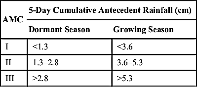
The value of CN depends on the antecedent moisture condition (AMC), hydrological soil group, hydrologic surface condition, and land use.

AMC is categorized into three levels: AMC I (for dry condition of soil), AMC II (for normal or average condition of soil), and AMC III (for wet condition of soil); which depends upon 5-day cumulative antecedent rainfall (Table 12.7).

Based on the AMC conditions, CN values will be adjusted. The following expressions will be used for converting the CN_II values into CN_I and CN_III.

${CN}_{I} = \frac{{CN}_{II}}{2.3 - 0.013 {CN}_{II}}$ ${CN}_{I} = \frac{{CN}_{II}}{2.3 - 0.013 {CN}_{II}}$

(12.33)

Table 12.7

Antecedent Soil Moisture Conditions (McCuen, 1989)

AMC	5-Day Cumulative Antecedent Rainfall (cm)
AMC	Dormant Season	Growing Season
I	<1.3	<3.6
II	1.3–2.8	3.6–5.3
III	>2.8	>5.3

${CN}_{III} = \frac{{CN}_{II}}{0.43 + 0.0057 {CN}_{II}}$ ${CN}_{III} = \frac{{CN}_{II}}{0.43 + 0.0057 {CN}_{II}}$

(12.34)

where CN_I and CN_III are the CN values corresponding to AMC I and AMC III.

The hydrological soil group and hydrological condition of watershed surface can be categorized as per Tables 12.8 and 12.9, respectively.

The values of CN for normal AMC and the hydrological surface condition and soil group are summarized in Table 12.10.

Table 12.8

Description of Hydrologic Groups

Hydrologic Soil Group	Minimum Infiltration Rate (cm/h)
A	0.76–1.14
B	0.38–0.76
C	0.13–0.38
D	0–0.13

Table 12.9

Classification of Woods (USDA, 1972)

S. No.	Vegetation Condition	Hydrologic Condition
1	Heavily grazed or regularly burned. Litter, small trees, and brush are destroyed	Poor
2	Grazed but not burned. Some litter exists, but these woods not protected	Fair
3	Protected from grazing and litter and shrubs cover the soil	Good

Table 12.10

Runoff Curve Number (CN) for Hydrologic Soil Cover Complex

Land Use	Cover	Hydrologic Condition	AMC II
	Treatment/Practice		I_a = 0.3S			I_a = 0.1S
	Treatment/Practice		A	B	C	D
Cultivated	Straight	Fair	76	86	90	93
Cultivated	Contoured	Poor	70	79	84	88
Cultivated	Contoured	Good	65	75	82	86
Cultivated	Contoured and terraced	Poor	66	74	80	82
Cultivated	Contoured and terraced	Good	62	71	77	81
Cultivated	Bunded	Poor	67	75	81	83
Cultivated	Bunded	Good	59	69	76	79
Cultivated	Paddy		95	95	95	95
Orchards	–	Poor	39	53	67	71
Orchards	–	Good	41	55	69	73
Forest	–	Poor	26	40	58	61
		Fair	28	44	60	64
		Good	33	47	64	67
Pasture	–	Poor	68	79	86	89
		Fair	49	69	79	84
		Good	39	61	74	80
Wasteland	–	–	71	80	85	88
Roads (dirt)	–	–	73	83	88	90
Hard surface area	–	–	77	86	91	93

Considering the land use, land treatment, hydrologic condition, and hydrologic soil group, the value of CN corresponding to the AMC II condition is selected (Table 12.10) and converted into CN_I, CN_II, or CN_III (Eqs. 12.33 and 12.34) as per the actual AMC condition based on 5-day cumulative antecedent rainfall. This CN value is converted into maximum potential retention using Eq. (12.32) followed by the estimation of direct runoff, Q using Eqs. (12.30) and (12.31). Once the value of Q is estimated, the effective rainfall R_e can be determined using Eq. (12.27).

12.2.5. Upward Flux of Water to the Root Zone Depth or Capillary Rise (U)

The upward flux of water to the root zone or capillary rise depends on the depth of water table. In many cases in tropical semiarid to subhumid regions, the groundwater table is very deep as compared to the root zone depth, therefore, the term U can be neglected.

12.2.6. Software for Irrigation Scheduling

For the algorithm described for irrigation scheduling using the water balance method, software for the irrigation scheduling has been developed using the Microsoft Office-Excel platform. A print screen of the software is depicted in Fig. 12.2.

12.3. Warabandi Scheduling

In general, an irrigation project is designed to cover the full command area with certain prefixed irrigation intensity, considering the equitable distribution norms. However, in practice, due to various reasons the head reach farmers get more water, whereas the tail reach farmers do not get sufficient irrigation supply most of the time. To overcome this unequitable distribution of water supply, a Warabandi scheduling program is developed, considering the irrigation water availability in the reservoir so that all farmers in the command area can be benefitted. Under this program, the turns are allocated to each farmer according to their land holdings. Considering this philosophy, this chapter elaborates the procedure adopted in the Warabandi Scheduling.

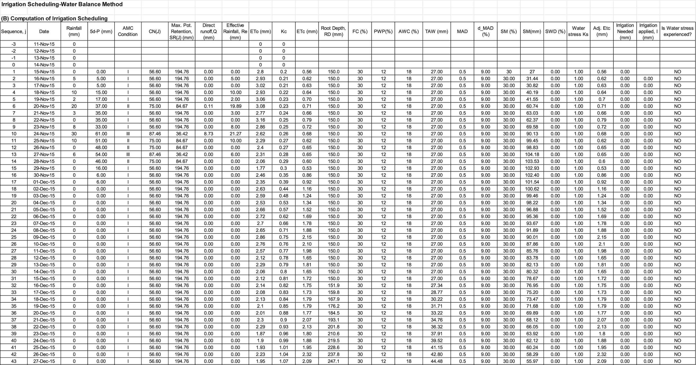
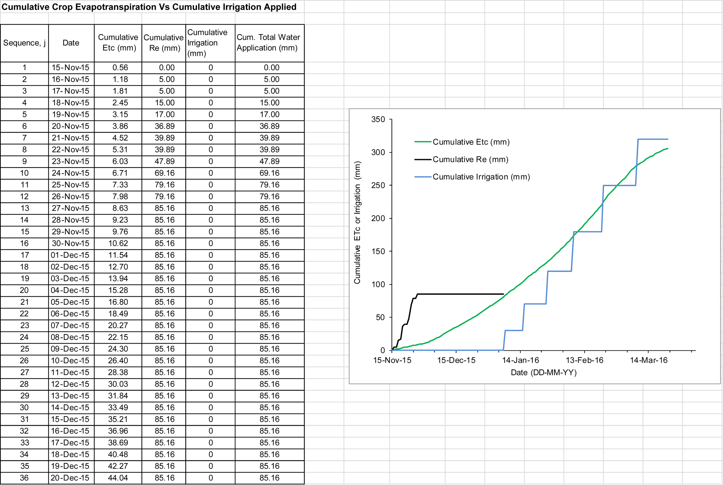
Figure 12.2 Print screen of the Irrigation scheduling software on EXCEL platform. (A) Data input sheet. (B) Computational sheet. (C) Summary sheet. CCA, culturable command area; ICA, irrigated command area.

12.3.1. Definition of Warabandi/Barabandi

Warabandi, also called “barabandi,” is a rotational system of equitable water distribution by turn in proportion to the land holding within an outlet command. “Wara” means “turn” and “bandi” means “fixation,” i.e., warabandi or barabandi means “fixation of turns,” which is adopted according to a predetermined schedule clearly specifying the “day, time, and duration” of supply of water to each irrigator or farmer. It is just not distributing water flowing inside a channel according to a roaster, but is an integrated water management system extending from the source to the farm gate. The need to equitably distribute the limited water resource available in an irrigation system among all the legitimate water users in that system is the basic premise underlying the concept of warabandi (Singh, 1980).

12.3.2. Indicators of Good Water Distribution System

Some important indicators of a successful distribution system are as follows:

1. Appropriateness as per the area and water availability;

2. Equity: (a) between large and small farmers, (b) between locations, i.e., from head to tail, and (c) equitability of time as per land holdings; and

3. Predictability: (a) adequacy, (b) timeliness, (c) flexibility, (d) incentive to users, and (e) less scope of malpractices

12.3.3. Water Distribution Methods

Water distribution methods under gravity flow irrigation can be broadly classified as: (1) flexible and (2) rigid method. These methods are briefly explained as under:

1. Flexible methods: This method involves much flexibility in demand as well as in operation and can be further classified as: (a) on-demand method, (b) modified demand method, and (c) continuous method.

Among the three methods, the first two are not in practice in Rajasthan as these methods need a huge canal section to cope with the undecided or unscheduled demand at a single point of time. Besides this the continuous method is being adopted in the projects, where water is available in ample quantity. In the continuous method, there is no control and water is wasted on the one hand and on the other hand those in need are deprived due to the lack of proper management.

2. Rigid methods: These methods do not allow the flexibility. The supply in these methods is controlled and the water distribution is based on the predetermined schedule or plan, which is strictly to be followed with rigidity.

Under this method, mainly the rotational water distribution is covered, which is named warabandi. Warabandi too is only practised in some of the projects in Western Rajasthan, viz., Ganga Canal, Bhakhra Canal, and Indira Gandhi Canal. This practice of warabandi in these canal systems satisfactorily works for effective water management and equitable distribution.

12.3.4. Enforcement in Warabandi

In the case that the Divisional Irrigation Officer is of the opinion that the distribution of irrigation water in a chak is not being ensured equitably and economically and warabandi is essential, he may enforce the same under the provisions of water policies after giving adequate publicity (Rajasthan Irrigation and Drainage Act, 1955). The breach of such warabandi will be an offense punishable under the Act. In spite of the enforcement policy, warabandi scheduling has a limitation for its implementation (Sanimer et al., 2011).

12.3.5. Systems of Warabandi

Warabandi can be categorized in view of the system of water distribution as: (1) nakewar warabandi, (2) goal warabandi, and (3) khatewar warabandi.

12.3.6. Forms of Warabandi

Warabandi can be planned in three forms as far as scheduling is concerned:

1. Noncontinuous warabandi (gili-gili warabandi),

2. Continuous warabandi (weekly temporary gili-sukhi warabandi), and

3. Continuous warabandi (weekly permanent)

Weekly permanent warabandi is prevalent in the Ganga canal, Bhakhra canal, and Indira Gandhi Nahar Pariyojna (IGNP).

12.4. Process of Warabandi

Warabandi is a continuous rotation of water in which one complete cycle of rotation lasts 7 days (or in some instances, 10.5 days), and each farmer in the watercourse receives water during one turn in this cycle for an already fixed length of time. The cycle begins at the head and proceeds to the tail of the watercourse, and during each turn, the farmer has the right to use all the water flowing in the watercourse. Each year, preferably at the canal closure, the warabandi cycle or roster is rotated by 12 h to give relief to those farmers who had their turns during the night in the preceding year's schedule. The time duration for each farmer is proportional to the size of the farmer's landholding to be irrigated within the particular watercourse command area. A certain time allowance is also given to farmers who need to be compensated for conveyance time, but no compensation is specifically made for seepage losses along the watercourse. Therefore the water users have to maintain the watercourse in good condition as successful warabandi operation relies heavily on the hydraulic performance of the conveyance system. These conditions, and those who are responsible for maintaining these conditions, together with an expected behavioral pattern among both the agency staff and the farmers, form the concept of a warabandi system.

12.4.1. Data Requirement for Warabandi Roaster

For the preparation of warabandi plan for a particular chak, the chak plan (map of chak) is needed with the following information details within it:

1. Details of culturable command area (CCA),

2. Sanctioned alignment of watercourse duly marked on the chak plan,

3. Geometry of the watercourse,

4. List of farmers along with the details of holdings,

5. Location of naka points on the watercourse,

6. Filling time (bharai) from one naka to other, and

7. Depletion time (jharai)

12.4.2. Formulation of Warabandi Schedule

The warabandi schedule is framed to form and maintain water distribution schedules for watercourses, generally assigned by the Irrigation Department. Theoretically, in calculating the duration of the warabandi turn given to a particular farm plot, some allowance is added to compensate for the time taken by the flow to fill that part of the watercourse leading to the farm plot. This is called bharai or watercourse “filling time.” Similarly, in some cases, a farm plot may continue to receive water from a filled portion of the watercourse even when it is closed from upstream to divert water to another farm or another part of the watercourse command. This is called jharai or “draining time,” and is deducted from the turn duration of that farm plot.

The warabandi roaster is prepared to be completed in a period of 7 days, i.e., 168 h (7 × 24 = 168). The turn should start at the head of watercourse at 6.00 a.m. on Monday and will end on 6.00 a.m. on the next Monday after completing 168 h. The calculation of time allocated per unit area of the chak and the time further allocated to the individual farmer for his land holding is computed by using the following formulae:

1. Unit irrigation time for flow per unit area under the watercourse (TU) in hours per hectare

$TU = (168 - TF + TD) / CCA$ $TU = (168 - TF + TD) / CCA$

(12.35)

where TU is the unit time for flow per unit area under the watercourse (h/ha), TF is filling time (h), TD is the draining time (h), and CCA is the culturable command area under the watercourse (ha). The value of TU should be the same for all the farmers in the watercourse.

2. Farmer's warabandi turn time (T_t): It gives the total time of run for the individual farmer with respect to the size of his holding. It is determined using the following formula:

$T_{t} = (TU \times A_{C h a k}) + Δ TF - Δ TD$ $T_{t} = (TU \times A_{C h a k}) + Δ TF - Δ TD$

(12.36)

where T_t is the turn time for irrigating individual's farm area or chak (h), A_Chak is the area of the chak of the farmer (ha), ΔTF is the filling time or bharai (h) between two consecutive naka, and TD is the draining time, or jharai (h) between two consecutive naka. Bharai (ΔTF) is generally zero in the case of the last farmer in the watercourse, and jharai (ΔTD) is zero for all the farmers excepting the last farmer in the watercourse.

As per the practice in IGNP, where agricultural plots are well planned as it is distributed after the completion of project, the filling time has been standardized at 20 min per Murrobba (i.e., 825 ft) (i.e., 0.21 m/s) for unlined and 10 min per 825 ft (i.e., 0.42 m/s) for lined water courses. For draining time, two times of the filling time is generally considered.

Since the existing irrigation project does not have planned agricultural plots, this criterion could not be considered, although the range would be same. In the present study, the draining time will be estimated, based on the actual measured flow velocity and length of watercourse in consecutive outlets (naka). The formula used for filling time is:

$Δ TF = \frac{Δ L}{60 \cdot \bar{v}}$ $Δ TF = \frac{Δ L}{60 \cdot \bar{v}}$

(12.37)

where ΔTF is the filling time or bharai (h) between two consecutive times, naka (min), ΔL is the length between consecutive naka (m), and

\bar{v}

$\bar{v}$

is average measured velocity (m/s). Here, ΔTD is computed as:

$Δ TD = 2 \cdot Δ TF$ $Δ TD = 2 \cdot Δ TF$

(12.38)

The turns are fixed on the basis of “first come first served basis” from head downward.

A sample warabandi program for the project for watercourse is given as follows along with watercourse and chak plan (Figs. 12.3 and 12.4).

12.5. Concluding Remarks

In the chapter, two aspects of irrigation distribution have been discussed. The first aspect focuses on the irrigation scheduling process, whereas the second one deals with the warabandi scheduling.

Irrigation scheduling is one of the important aspects of irrigation delivery through which time and magnitude of irrigation delivery to the farm land can be fixed. For irrigation scheduling, two methods were presented: (1) FAO (1989) and (2) water balance method. The former approach provides a general idea of irrigation scheduling, whereas the latter approach is quite comprehensive and is based on daily soil moisture balance. The latter approach can also be utilized on a real-time basis by using the forecasted temperature and rainfall to get timely measured irrigation requirements for the field.

Generally, an irrigation project is designed to cover the full command area with certain prefixed irrigation intensity, considering the equitable distribution norms. However, in practice, due to various reasons, the head reach farmers get more water, whereas the tail reach farmers simply wait for water delivery. It can also be understood using the term irrigation intensity. If the project is designed for 50% irrigation intensity, then 50% of CCA will get irrigation supply through the project though equitably distributed in CCA. However, in reality, the upper reaches of the distribution system achieves 100% irrigation intensity, which means that farmers get water for their full agriculture land, whereas in the lower reaches due to excess supply in the upper reaches, the canal water does not reach and the observed irrigation intensity is either almost zero or less than the designed one. To overcome this nonequitable distribution of water, warabandi scheduling is required. It is important to note that the success of the warabandi scheduling or program largely depends on the discipline among the farmers, for which sometimes enforcement is done.

Figure 12.3 Map showing a small watercourse and chak plan. CCA, culturable command area; ICA, irrigated command area.

Figure 12.4 Map showing a large watercourse and chak plan. CCA, culturable command area; ICA, irrigated command area.

..................Content has been hidden....................

You can't read the all page of ebook, please click here login for view all page.

Table of Contents for Chapter 12. Irrigation Scheduling

Create new playlist

Sign In

Sign Up