Search in book...
Toggle Font Controls
Create new playlist

Name your new playlist

Playlist description (optional)
Sign In

Email address

Password

Forgot Password?

or

Continue with Facebook

Continue with Google
Sign Up

Full Name

Email address

Confirm Email Address

Password

or

Continue with Facebook

Continue with Google

Chapter 5

Estimation of Lake Evaporation and Potential Evapotranspiration

Abstract

Evaporation is one of the major losses from lakes and reservoirs, which requires to be accounted for water budgeting. When there is no instrumentation available for the direct measurement of lake evaporation, it becomes necessary to use models for its estimation. The Penman method is considered as one of the most reliable methods for estimating lake evaporation and is discussed in sufficient detail in the chapter. Besides estimating the evaporation loss from reservoirs, estimation of reference crop evapotranspiration or potential evapotranspiration is also required, which forms the basis of estimating the crop water requirement for irrigation planning. In this chapter, the Penman–Monteith method and ASCE-EWRI Standardized Penman–Monteith equation are discussed in detail along with the Hargreaves method for limited meteorological data availability.

Keywords

ASCE-EWRI standardized Penman–Monteith equation; Hargreaves method; Lake evaporation; Penman method; Penman–Monteith method; Potential evapotranspiration; Reference crop evapotranspiration

For planning of a reservoir project, evaporation plays an important component in the hydrological budget. Evaporation is one of the major losses from lakes and reservoirs, and its accounting is therefore important. Evaporation losses can directly be measured using the evaporation pan; however, at many reservoir locations or sites, it is not installed. When there is no instrumentation available for the direct measurement of lake evaporation, it becomes necessary to use models for its estimation. Here, the Penman method is considered as one of the most reliable methods for estimating lake evaporation. Similarly, for planning of irrigation projects, crop water requirement is the most important parameter, which determines the irrigation water requirement for the proposed command area as per the cropping pattern, followed by assessment of net water required in the reservoir or diversion head for meeting the irrigation supply. For estimating the crop water requirement, the reference crop evapotranspiration or potential evapotranspiration is required to be estimated first, for which various methods have been developed. However, the Penman–Monteith method and ASCE-EWRI Standardized Penman–Monteith equation are used frequently. These methods are described here. One of the requirements of these methods is the availability of good-quality meteorological data. When meteorological data are limited, the Hargreaves method can be used, which is also discussed in this chapter.

5.1. Estimation of Lake Evaporation

The Penman equation (Penman, 1948), a well-known combination equation (i.e., combination of energy balance and an aerodynamic formula) can be expressed as follows:

$E = \frac{Δ}{Δ + γ} \cdot \frac{R_{n}}{λ} + \frac{γ}{Δ + γ} \cdot E_{a}$ $E = \frac{Δ}{Δ + γ} \cdot \frac{R_{n}}{λ} + \frac{γ}{Δ + γ} \cdot E_{a}$

(5.1)

where E = evaporation (mm/d); λ = the latent heat of vaporization (MJ/kg) = 2.45 MJ/kg;

Δ = the slope of the saturated vapor pressure curve (i .e ., \partial e_{s} / \partial T) (kPa / ° C)

$Δ = the slope of the saturated vapor pressure curve (i .e ., \partial e_{s} / \partial T) (kPa / ° C)$

; e_s = the saturated vapor pressure (kPa); T = the temperature (°C); R_n = the net radiation flux (MJ/m²/d); G = the sensible heat flux into soil (MJ/m²/d); γ = the psychometric constant (kPa/°C) = 0.059 kPa/°C; E_a = the vapor transport flux (mm/d) = f {u₂, (e_s–e_a)}; u₂ = the wind speed (m/s); and e_a = the actual vapor pressure (kPa). The variables used in Eq. (5.1) can be estimated from various relationships summarized in Table 5.1.

Utilizing the meteorological data, lake evaporation can be estimated using Eq. (5.1). Once it is estimated, the net evaporation loss from the lake is computed and converted into the volumetric unit using Eqs. (5.2) and (5.3).

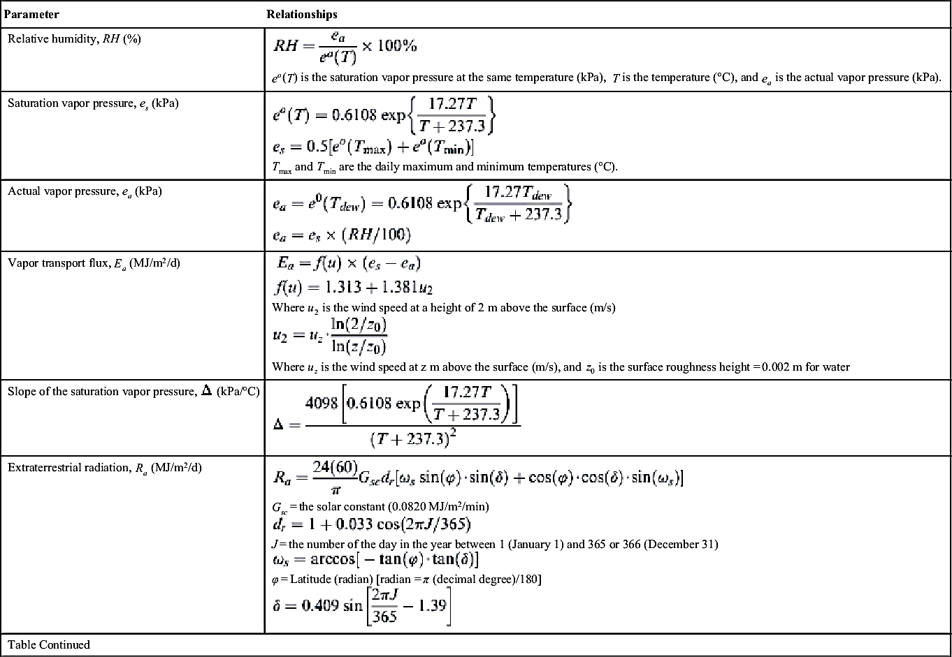
Table 5.1

Auxiliary Equations Used for Penman Method

Parameter	Relationships
Relative humidity, RH (%)	$R H = \frac{e_{a}}{e^{o} (T)} \times 100 %$ $R H = \frac{e_{a}}{e^{o} (T)} \times 100 %$ e^o(T) is the saturation vapor pressure at the same temperature (kPa), T is the temperature (°C), and e_a is the actual vapor pressure (kPa).
Saturation vapor pressure, e_s (kPa)	$e^{o} (T) = 0.6108 \exp {\frac{17.27 T}{T + 237.3}}$ $e^{o} (T) = 0.6108 \exp {\frac{17.27 T}{T + 237.3}}$ $e_{s} = 0.5 [e^{o} (T_{\max}) + e^{o} (T_{\min})]$ $e_{s} = 0.5 [e^{o} (T_{\max}) + e^{o} (T_{\min})]$ T_max and T_min are the daily maximum and minimum temperatures (°C).
Actual vapor pressure, e_a (kPa)	$e_{a} = e^{0} (T_{d e w}) = 0.6108 \exp {\frac{17.27 T_{d e w}}{T_{d e w} + 237.3}}$ $e_{a} = e^{0} (T_{d e w}) = 0.6108 \exp {\frac{17.27 T_{d e w}}{T_{d e w} + 237.3}}$ $e_{a} = e_{s} \times (R H / 100)$ $e_{a} = e_{s} \times (R H / 100)$
Vapor transport flux, E_a (MJ/m²/d)	$\begin{matrix} E_{a} = f (u) \times (e_{s} - e_{a}) \\ f (u) = 1.313 + 1.381 u_{2} \end{matrix}$ $\begin{matrix} E_{a} = f (u) \times (e_{s} - e_{a}) \\ f (u) = 1.313 + 1.381 u_{2} \end{matrix}$ Where u₂ is the wind speed at a height of 2 m above the surface (m/s) $u_{2} = u_{z} \cdot \frac{\ln (2 / z_{0})}{\ln (z / z_{0})}$ $u_{2} = u_{z} \cdot \frac{\ln (2 / z_{0})}{\ln (z / z_{0})}$ Where u_z is the wind speed at z m above the surface (m/s), and z₀ is the surface roughness height = 0.002 m for water
Slope of the saturation vapor pressure, 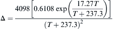$Δ$ $Δ$ (kPa/°C)	$Δ = \frac{4098 [0.6108 \exp (\frac{17.27 T}{T + 237.3})]}{{(T + 237.3)}^{2}}$ $Δ = \frac{4098 [0.6108 \exp (\frac{17.27 T}{T + 237.3})]}{{(T + 237.3)}^{2}}$
Extraterrestrial radiation, R_a (MJ/m²/d)	$R_{a} = \frac{24 (60)}{π} G_{s c} d_{r} [ω_{s} \sin (φ) \cdot \sin (δ) + \cos (φ) \cdot \cos (δ) \cdot \sin (ω_{s})]$ $R_{a} = \frac{24 (60)}{π} G_{s c} d_{r} [ω_{s} \sin (φ) \cdot \sin (δ) + \cos (φ) \cdot \cos (δ) \cdot \sin (ω_{s})]$ G_sc = the solar constant (0.0820 MJ/m²/min) $d_{r} = 1 + 0.033 \cos (2 π J / 365)$ $d_{r} = 1 + 0.033 \cos (2 π J / 365)$ J = the number of the day in the year between 1 (January 1) and 365 or 366 (December 31) $ω_{s} = \arccos [- \tan (φ) \cdot \tan (δ)]$ $ω_{s} = \arccos [- \tan (φ) \cdot \tan (δ)]$ φ = Latitude (radian) [radian = π (decimal degree)/180] $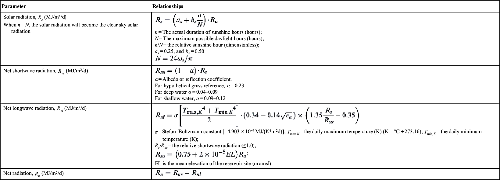δ = 0.409 \sin [\frac{2 π J}{365} - 1.39]$ $δ = 0.409 \sin [\frac{2 π J}{365} - 1.39]$
Table Continued

Parameter	Relationships
Solar radiation, R_s (MJ/m²/d) When n = N, the solar radiation will become the clear sky solar radiation	$R_{s} = (a_{s} + b_{s} \frac{n}{N}) \cdot R_{a}$ $R_{s} = (a_{s} + b_{s} \frac{n}{N}) \cdot R_{a}$ n = The actual duration of sunshine hours (hours); N = The maximum possible daylight hours (hours); n/N = the relative sunshine hour (dimensionless); a_s = 0.25, and b_s = 0.50 $N = 24 ω_{s} / π$ $N = 24 ω_{s} / π$
Net shortwave radiation, R_ns (MJ/m²/d)	$R_{n s} = (1 - α) \cdot R_{s}$ $R_{n s} = (1 - α) \cdot R_{s}$ α = Albedo or reflection coefficient. For hypothetical grass reference, α = 0.23 For deep water α = 0.04–0.09 For shallow water, α = 0.09–0.12
Net longwave radiation, R_nl (MJ/m²/d)	$R_{n l} = σ [\frac{{T_{\max, K}}^{4} + {T_{\min, K}}^{4}}{2}] \cdot (0.34 - 0.14 \sqrt{e_{a}}) \times (1.35 \frac{R_{s}}{R_{s o}} - 0.35)$ $R_{n l} = σ [\frac{{T_{\max, K}}^{4} + {T_{\min, K}}^{4}}{2}] \cdot (0.34 - 0.14 \sqrt{e_{a}}) \times (1.35 \frac{R_{s}}{R_{s o}} - 0.35)$ σ = Stefan–Boltzmann constant [=4.903 × 10⁻⁹ MJ/(K⁴m²d)]; T_max,K = the daily maximum temperature (K) (K = °C + 273.16); T_min,K = the daily minimum temperature (K); R_s/R_so = the relative shortwave radiation (≤1.0); $R_{s o} = (0.75 + 2 \times 10^{- 5} E L) R_{a}$ $R_{s o} = (0.75 + 2 \times 10^{- 5} E L) R_{a}$ ; EL is the mean elevation of the reservoir site (m amsl)
Net radiation, R_n (MJ/m²/d)	$R_{n} = R_{n s} - R_{n l}$ $R_{n} = R_{n s} - R_{n l}$

$E_{l a k e} (mm) = (E - P)$ $E_{l a k e} (mm) = (E - P)$

(5.2)

$E_{l a k e} (MCM) = 10^{- 5} \times (E - P) \times \bar{A}$ $E_{l a k e} (MCM) = 10^{- 5} \times (E - P) \times \bar{A}$

(5.3)

where E is the evaporation (mm), P is the rainfall over the lake or reservoir (mm), and

\bar{A}

$\bar{A}$

is the average water surface area of the reservoir during the period (ha).

Example 5.1:

The station located at a latitude of 28°34′47.064″ N at an elevation of 630 m above mean sea level. The climatic data observed on January 1 are as follows:

Maximum temperature, T_max = 15°C; minimum temperature, T_min = 8°C; dew point temperature, T_dew = 10.44°C; and wind speed at 2 m height, u₂ = 1.25 m/s.

Estimate the reference crop evapotranspiration using the Penman equation.

Solution:

Variable	Unit	Equation	Value
Latitude	degree		28.57974
Elevation	m		630
T_max	°C		15
T_min	°C		8
T_dew	°C		10.44
u₂	m/s		1.25
Sunshine duration, n	h		8
T_mean	°C	=0.5(T_max + T_min)	11.5
Albedo, α			0.23
Psychometric constant, γ	kPa/°C		0.059
Saturation vapor pressure, $\begin{matrix} e_{z}^{o} \end{matrix}$ $\begin{matrix} e_{z}^{o} \end{matrix}$	kPa	$e^{o} (T) = 0.6108 \exp {\frac{17.27 T}{T + 237.3}}$ $e^{o} (T) = 0.6108 \exp {\frac{17.27 T}{T + 237.3}}$ $e_{s} = 0.5 [e^{o} (T_{\max}) + e^{o} (T_{\min})]$ $e_{s} = 0.5 [e^{o} (T_{\max}) + e^{o} (T_{\min})]$ T_max and T_min are the daily max and minimum temperatures (°C).	1.389058
Actual vapor pressure, $\begin{matrix} e_{z}^{o} \end{matrix}$ $\begin{matrix} e_{z}^{o} \end{matrix}$	kPa	$e_{a} = e^{0} (T_{d e w}) = 0.6108 \exp {\frac{17.27 T_{d e w}}{T_{d e w} + 237.3}}$ $e_{a} = e^{0} (T_{d e w}) = 0.6108 \exp {\frac{17.27 T_{d e w}}{T_{d e w} + 237.3}}$ $e_{a} = e_{s} \times (R H / 100)$ $e_{a} = e_{s} \times (R H / 100)$	1.264641
Vapor pressure deficit	kPa	= $\begin{matrix} e_{z}^{o} - e_{z} \end{matrix}$ $\begin{matrix} e_{z}^{o} - e_{z} \end{matrix}$	0.124416
Wind function, f(u)		= $\begin{matrix} 6.43 (a_{w} + b_{w} u_{2}) \end{matrix}$ $\begin{matrix} 6.43 (a_{w} + b_{w} u_{2}) \end{matrix}$	7.555
The vapor transport flux, E_a	MJ/m²/d	$\begin{matrix} E_{a} = f (u) \times (e_{s} - e_{a}) \\ f (u) = 1.313 + 1.381 u_{2} \end{matrix}$ $\begin{matrix} E_{a} = f (u) \times (e_{s} - e_{a}) \\ f (u) = 1.313 + 1.381 u_{2} \end{matrix}$ Where u₂ is the wind speed at a height of 2 m above the surface (m/s) $u_{2} = u_{z} \cdot \frac{\ln (2 / z_{0})}{\ln (z / z_{0})}$ $u_{2} = u_{z} \cdot \frac{\ln (2 / z_{0})}{\ln (z / z_{0})}$ Where u_z is the wind speed at z m above the surface (m/s), and z₀ is the surface roughness height = 0.002 m for water.	0.940
Table Continued

Variable	Unit	Equation	Value
J Corresponding to January 1			1
The latitude, φ	radian	radian = π (decimal degree)/180	0.498811
The inverse relative distance of the earth from the sun, d_r		$d_{r} = 1 + 0.033 \cos (2 π J / 365)$ $d_{r} = 1 + 0.033 \cos (2 π J / 365)$	1.032995
The sunset hour angle ω_s is	radian	$ω_{s} = \arccos [- \tan (φ) \cdot \tan (δ)]$ $ω_{s} = \arccos [- \tan (φ) \cdot \tan (δ)]$	1.337724
The solar declination, δ	radian	$δ = 0.409 \sin [\frac{2 π J}{365} - 1.39]$ $δ = 0.409 \sin [\frac{2 π J}{365} - 1.39]$	−0.40101
The maximum possible sunshine duration, N	h	$N = 24 ω_{s} / π$ $N = 24 ω_{s} / π$	10.21946
The relative sunshine duration, n/N	–	=n/N	0.78282
The extra-terrestrial radiation, R_a	MJ/m²/d	$R_{a} = \frac{24 (60)}{π} G_{s c} d_{r} [ω_{s} \sin (φ) \cdot \sin (δ) + \cos (φ) \cdot \cos (δ) \cdot \sin (ω_{s})]$ $R_{a} = \frac{24 (60)}{π} G_{s c} d_{r} [ω_{s} \sin (φ) \cdot \sin (δ) + \cos (φ) \cdot \cos (δ) \cdot \sin (ω_{s})]$	20.84294
The solar radiation, R_s	MJ/m²/d	$R_{s} = (a_{s} + b_{s} \frac{n}{N}) \cdot R_{a}$ $R_{s} = (a_{s} + b_{s} \frac{n}{N}) \cdot R_{a}$ n = the actual duration of sunshine hours (h); N = the maximum possible daylight hours (h); n/N = the relative sunshine hour (dimensionless); a_s = 0.25, and b_s = 0.50 $N = 24 ω_{s} / π$ $N = 24 ω_{s} / π$	13.36888
The clear-sky solar radiation, R_so	MJ/m²/d	$R_{s o} = (0.75 + 2 \times 10^{- 5} E L) R_{a}$ $R_{s o} = (0.75 + 2 \times 10^{- 5} E L) R_{a}$	15.89483
The net shortwave radiation, R_ns	MJ/m²/d	$R_{n s} = (1 - α) \cdot R_{s}$ $R_{n s} = (1 - α) \cdot R_{s}$ $α = the Aalbedo or reflection coefficient$ $α = the Aalbedo or reflection coefficient$ For hypothetical grass reference, $α = 0.23$ $α = 0.23$ For deep water $α = 0.04 to 0.09$ $α = 0.04 to 0.09$ For shallow water, $α = 0.09 to 0.12$ $α = 0.09 to 0.12$	10.29403
T_max	K	K = °C + 273.16	288.16
T_min	K	K = °C + 273.16	281.16
The net longwave radiation, R_nl	MJ/m²/d	$R_{n l} = σ [\frac{{T_{\max, K}}^{4} + {T_{\min, K}}^{4}}{2}] \cdot (0.34 - 0.14 \sqrt{e_{a}}) \times (1.35 \frac{R_{s}}{R_{s o}} - 0.35)$ $R_{n l} = σ [\frac{{T_{\max, K}}^{4} + {T_{\min, K}}^{4}}{2}] \cdot (0.34 - 0.14 \sqrt{e_{a}}) \times (1.35 \frac{R_{s}}{R_{s o}} - 0.35)$	4.62057
The net radiation, R_n	MJ/m²/d	$R_{n} = R_{n s} - R_{n l}$ $R_{n} = R_{n s} - R_{n l}$	5.67347
The soil heat flux, G	MJ/m²/d		0.0
The reference crop evapotranspiration, $\begin{matrix} λ E \end{matrix}$ $\begin{matrix} λ E \end{matrix}$	MJ/m²/d	=E/2.45	3.7970
The reference crop evapotranspiration, $\begin{matrix} E T_{o} \end{matrix}$ $\begin{matrix} E T_{o} \end{matrix}$	mm/d	$E = \frac{Δ}{Δ + γ} \cdot \frac{R_{n}}{λ} + \frac{γ}{Δ + γ} \cdot E_{a}$ $E = \frac{Δ}{Δ + γ} \cdot \frac{R_{n}}{λ} + \frac{γ}{Δ + γ} \cdot E_{a}$	1.5492

5.2. Estimation of Reference Crop Evapotranspiration

5.2.1. FAO-56 and ASCE-EWRI Method

Accuracy of the reference crop evapotranspiration (ET_o) is vital for the design and planning of irrigation projects, as it forms the basic input for the estimation of irrigation requirement. For estimating ET₀, perhaps the most acceptable method is the FAO-56 Reference Crop evapotranspiration method, which is discussed here. This method uses the various climatic parameters generally recorded at climatic or weather stations. The governing equation for estimating ET_o is as follows (Monteith, 1965; Allen et al., 1998).

$E T_{o} = \frac{0.408 Δ (R_{n} - G) + γ \frac{900}{T + 273} u_{2} (e_{z}^{0} - e_{z})}{Δ + γ (1 + 0.34 u_{2})}$ $E T_{o} = \frac{0.408 Δ (R_{n} - G) + γ \frac{900}{T + 273} u_{2} (e_{z}^{0} - e_{z})}{Δ + γ (1 + 0.34 u_{2})}$

(5.4)

In Eq. (5.4) ET_o = the grass reference ET (mm/d); R_n = the net radiation (MJ/m²/d); G = the sensible heat exchange from the surface to the soil or water (MJ/m²/d); T = the mean daily temperature (°C);

Δ = the slope of the saturation vapor pressure versus temperature (kPa/ ° C)

$Δ = the slope of the saturation vapor pressure versus temperature (kPa/ ° C)$

; γ = the psychometric constant (kPa/°C); u₂ = the mean 24-h wind speed at 2 m above the ground (m/s);

e_{z}^{o} = the saturation vapor pressure based on measurements at 1.5 - 2 .0 m (kPa)

$e_{z}^{o} = the saturation vapor pressure based on measurements at 1.5 - 2 .0 m (kPa)$

; e_z = the actual vapor pressure (kPa). This method (i.e., FAO-56) is more suitable for short grasses or crops.

For long or tall crops or grasses, the ASCE-EWRI standardized Penman–Monteith equation can be used (ASCE, 2005). The ASCE-EWRI equation for ET_o is expressed as follows:

$E T_{o} = \frac{0.408 Δ (R_{n} - G) + γ \frac{1600}{T + 273} u_{2} (e_{z}^{0} - e_{z})}{Δ + γ (1 + 0.38 u_{2})}$ $E T_{o} = \frac{0.408 Δ (R_{n} - G) + γ \frac{1600}{T + 273} u_{2} (e_{z}^{0} - e_{z})}{Δ + γ (1 + 0.38 u_{2})}$

(5.5)

The parameters appearing in Eqs. (5.4) and (5.5) can be determined using the auxiliary equations summarized in Table 5.2.

5.2.2. Hargreaves Method

Under limited climatic data, the Hargreaves method (Hargreaves and Samani, 1985; Hargreaves, 1994) can be satisfactorily used and is expressed as follows:

$E T_{o} = 0.0023 (T_{m e a n} + 17.8) {(T_{\max} - T_{\min})}^{0.5} \times (0.408 \times R_{a})$ $E T_{o} = 0.0023 (T_{m e a n} + 17.8) {(T_{\max} - T_{\min})}^{0.5} \times (0.408 \times R_{a})$

(5.6)

where ET_o is the reference evapotranspiration (mm/d); T_mean, T_max, and T_min are the daily mean, maximum, and minimum temperatures (°C), respectively; and R_a is the extraterrestrial radiation for each day (MJ/m²/d). The Hargreaves equation has a tendency to underpredict under high-wind-speed conditions (u > 3 m/s) and overpredict under conditions of high relative humidity. A detailed procedure for estimating the value of R_a is summarized in Section 5.2.1.

Example 5.2:

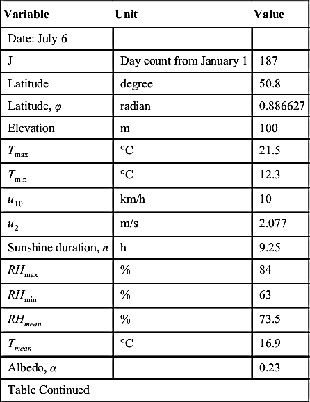
Determine ET_o for a given meteorological data measured on July 6 at station located at 50°48′ N and at 100 m above mean sea level using the Penman–Monteith method (FAO-56). The climatic data observed at the station are:

Maximum temperature, T_max = 21.5°C; minimum temperature, T_min = 12.3°C; RH_max = 84%; RH_min = 63%; wind speed at 10 m height = 10 km/h; and actual sunshine duration is 9.25 h.

Table 5.2

Auxiliary Equations Used for Penman–Montieth Method

Parameter	Relationships
Relative humidity, RH (%)	$R H = \frac{e_{a}}{e^{o} (T)} \times 100 %$ $R H = \frac{e_{a}}{e^{o} (T)} \times 100 %$ e^o(T) is the saturation vapor pressure at same temperature (kPa), T is the temperature (°C), and e_a is the actual vapor pressure (kPa)
Saturation vapor pressure, e_s (kPa)	$e^{o} (T) = 0.6108 \exp {\frac{17.27 T}{T + 237.3}}$ $e^{o} (T) = 0.6108 \exp {\frac{17.27 T}{T + 237.3}}$ $e_{s} = 0.5 [e^{o} (T_{\max}) + e^{o} (T_{\min})]$ $e_{s} = 0.5 [e^{o} (T_{\max}) + e^{o} (T_{\min})]$ T_max and T_min are the daily maximum and minimum temperatures (°C)
Actual vapor pressure, e_a (kPa)	$e_{a} = e^{0} (T_{d e w}) = 0.6108 \exp {\frac{17.27 T_{d e w}}{T_{d e w} + 237.3}}$ $e_{a} = e^{0} (T_{d e w}) = 0.6108 \exp {\frac{17.27 T_{d e w}}{T_{d e w} + 237.3}}$ $e_{a} = e_{s} \times (R H / 100)$ $e_{a} = e_{s} \times (R H / 100)$
U₂ (m/s)	$u_{2} = u_{z} \frac{4.87}{\ln (67.8 z - 5.42)}$ $u_{2} = u_{z} \frac{4.87}{\ln (67.8 z - 5.42)}$ Where u_z is the wind speed at z m above the surface (m/s) and z₀ is the surface roughness height = 0.002 m for water
Slope of the saturation vapor pressure, $Δ$ $Δ$ (kPa/°C)	$Δ = \frac{4098 [0.6108 \exp (\frac{17.27 T}{T + 237.3})]}{{(T + 237.3)}^{2}}$ $Δ = \frac{4098 [0.6108 \exp (\frac{17.27 T}{T + 237.3})]}{{(T + 237.3)}^{2}}$
Extraterrestrial radiation, R_a (MJ/m²/d)	$R_{a} = \frac{24 (60)}{π} G_{s c} d_{r} [ω_{s} \sin (φ) \cdot \sin (δ) + \cos (φ) \cdot \cos (δ) \cdot \sin (ω_{s})]$ $R_{a} = \frac{24 (60)}{π} G_{s c} d_{r} [ω_{s} \sin (φ) \cdot \sin (δ) + \cos (φ) \cdot \cos (δ) \cdot \sin (ω_{s})]$ G_sc = the solar constant (0.0820 MJ/m²/min) $d_{r} = 1 + 0.033 \cos (2 π J / 365)$ $d_{r} = 1 + 0.033 \cos (2 π J / 365)$ J = the number of the day in the year between 1 (January 1) and 365 or 366 (December 31) $ω_{s} = \arccos [- \tan (φ) \cdot \tan (δ)]$ $ω_{s} = \arccos [- \tan (φ) \cdot \tan (δ)]$ φ = Latitude (radian) [radian = π (decimal degree)/180] $δ = 0.409 \sin [\frac{2 π J}{365} - 1.39]$ $δ = 0.409 \sin [\frac{2 π J}{365} - 1.39]$
Solar radiation, R_s (MJ/m²/d) When n = N, the solar radiation will becomes the clear sky solar radiation.	$R_{s} = (a_{s} + b_{s} \frac{n}{N}) \cdot R_{a}$ $R_{s} = (a_{s} + b_{s} \frac{n}{N}) \cdot R_{a}$ n = The actual duration of sunshine hours (h); N = the maximum possible daylight hours (h); n/N = the relative sunshine hour (dimensionless); a_s = 0.25, and b_s = 0.50. $N = 24 ω_{s} / π$ $N = 24 ω_{s} / π$
Net shortwave radiation, R_ns (MJ/m²/d)	$R_{n s} = (1 - α) \cdot R_{s}$ $R_{n s} = (1 - α) \cdot R_{s}$ α = Albedo or reflection coefficient. For hypothetical grass reference, α = 0.23
Net longwave radiation, R_nl (MJ/m²/d)	$R_{n l} = σ [\frac{{T_{\max, K}}^{4} + {T_{\min, K}}^{4}}{2}] \cdot (0.34 - 0.14 \sqrt{e_{a}}) \times (1.35 \frac{R_{s}}{R_{s o}} - 0.35)$ $R_{n l} = σ [\frac{{T_{\max, K}}^{4} + {T_{\min, K}}^{4}}{2}] \cdot (0.34 - 0.14 \sqrt{e_{a}}) \times (1.35 \frac{R_{s}}{R_{s o}} - 0.35)$ σ = The Stefan–Boltzmann constant [=4.903 × 10⁻⁹ MJ/(K⁴m²d)] T_max,K = The daily maximum temperature (K) (K = °C + 273.16); T_min, K = the daily minimum temperature (K); and R_s/R_so = The relative shortwave radiation (≤1.0). $R_{s o} = (0.75 + 2 \times 10^{- 5} E L) R_{a}$ $R_{s o} = (0.75 + 2 \times 10^{- 5} E L) R_{a}$ Where R_so is the clear-sky solar radiation (MJ/m²/d), EL = the mean elevation of the reservoir site (m amsl).
Table Continued

Parameter	Relationships
Net radiation, R_n (MJ/m²/d)	$R_{n} = R_{n s} - R_{n l}$ $R_{n} = R_{n s} - R_{n l}$
Soil heat flux, G (MJ/m²/d)	For daily time periods, the magnitude of G averaged over 24 h beneath a fully vegetated grass or alfalfa reference surface is relatively small in comparison with R_n. Therefore for daily computation of ET₀, G can be ignored (i.e., G = 0). For water surface, G = 0
Psychometric constant, γ (kPa/°C)	$γ = \frac{c_{p} P}{ε λ} = 0.665 \times 10^{- 3} P$ $γ = \frac{c_{p} P}{ε λ} = 0.665 \times 10^{- 3} P$ Where, P is the atmospheric pressure (kPa), λ is the latent heat of vaporization (2.45 MJ/kg), c_p is the specific heat at constant pressure (1.013 × 10⁻³ MJ/kg/°C), and ε is the ratio of molecular weight of water vapor to that of dry air = 0.622 The simplified equation for relating the atmospheric pressure and elevation above the mean sea level can be given as follows: $P = 101.3 {(\frac{293 - 0.0065 E L}{293})}^{5.26}$ $P = 101.3 {(\frac{293 - 0.0065 E L}{293})}^{5.26}$

Solution:

The calculation procedure for the FAO-56 method—follows:

Variable	Unit	Value
Date: July 6
J	Day count from January 1	187
Latitude	degree	50.8
Latitude, φ	radian	0.886627
Elevation	m	100
T_max	°C	21.5
T_min	°C	12.3
u₁₀	km/h	10
u₂	m/s	2.077
Sunshine duration, n	h	9.25
RH_max	%	84
RH_min	%	63
RH_mean	%	73.5
T_mean	°C	16.9
Albedo, α		0.23
Table Continued

Variable	Unit	Value
Psychometric constant, γ	kPa/°C	0.0655
Δ	kPa/°C	0.12211
Saturation vapor pressure, $\begin{matrix} e_{z}^{o} \end{matrix}$ $\begin{matrix} e_{z}^{o} \end{matrix}$	kPa	1.9975
Actual vapor pressure, $\begin{matrix} e_{z}^{o} \end{matrix}$ $\begin{matrix} e_{z}^{o} \end{matrix}$	kPa	1.46815
Vapor pressure deficit	kPa	0.52933
The inverse relative distance of the earth from the sun, d_r		0.9670989
The sunset hour angle ω_s is	radian	2.108088
The solar declination, δ	radian	0.395436
The maximum possible sunshine duration, N	h	16.1046
The relative sunshine duration, n/N	–	0.57437
The extraterrestrial radiation, R_a	MJ/m²/d	41.088
The solar radiation, R_s	MJ/m²/d	22.072
The clear-sky solar radiation, R_so	MJ/m²/d	30.8984
The net shortwave radiation, R_ns	MJ/m²/d	16.9955
T_max	K	294.66
T_min	K	285.46
The net longwave radiation, R_nl	MJ/m²/d	3.63810
The net radiation, R_n	MJ/m²/d	13.35738
The soil heat flux, G	MJ/m²/d	0.0
Term1^a		0.6655
Term2^a		0.2239
Term3^a		0.2340
ET_o (Penman–Monteith)^b	mm/d	3.8005

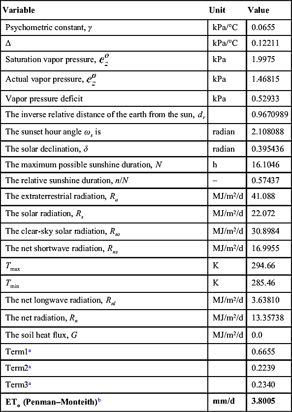
Therefore the estimated value of reference crop evapotranspiration using the Penman–Monteith method is 3.8005 mm/d.

Example 5.3:

Determine ET_o for a given meteorological data measured on July 6 at station located at 50°48′ N and at 100 m above mean sea level using the Hargreaves method. For this station, only daily maximum and daily minimum temperature data are available. The maximum and minimum temperatures are 21.5°C and 12.3°C, respectively.

Solution:

The computational procedure of Hargreaves method is as follows:

Parameters of the Hargreaves Method	Unit	Value
Date		July 6
J (day count since January 1)		187
T_mean	°C	16.9
T_max	°C	21.5
T_min	°C	12.3
Lat	degree	50.8
Lat	radian	0.886627
Elevation, z	m	100
Atmospheric pressure, P	kPa	0.0655
Psychometric constant,γ	kPa/°C	0.0656
The inverse relative distance of the Earth from the sun, d_r		0.9671
The sunset hour angle ω_s	radian	2.1080
The solar declination, δ	radian	0.3954
R_a	MJ/m²/d	41.0884
ET_o using the Hargreaves method	mm/d	4.0582

5.3. Concluding Remarks

Although a number of methods for computing evaporation have been published in the literature, this chapter is limited to the description of the methods that are frequently used for estimating evaporation from water bodies or lakes and reference crop evapotranspiration in irrigation planning. It is also suggested to use a method that is specifically developed for a particular site or region having specific climatic conditions.

..................Content has been hidden....................

You can't read the all page of ebook, please click here login for view all page.

Table of Contents for Chapter 5. Estimation of Lake Evaporation and Potential Evapotranspiration

Create new playlist

Sign In

Sign Up

Abstract

Keywords

5.1. Estimation of Lake Evaporation

5.2. Estimation of Reference Crop Evapotranspiration

5.2.1. FAO-56 and ASCE-EWRI Method

5.2.2. Hargreaves Method

5.3. Concluding Remarks

Table of Contents for
Chapter 5. Estimation of Lake Evaporation and Potential Evapotranspiration