This chapter presents the essential elements of catchment hydrology, especially analysis of rainfall up to the estimation of catchment yield and design-flood estimation, reservoir sizing, and preliminary analysis of reservoir sedimentation. The procedures used in the application of water budgeting, rainfall–runoff simulation, design-flood estimation, reservoir inflow, reservoir sizing, reservoir operation, and sedimentation for hydrological investigations required for irrigation planning are detailed with worked examples. A statistical method for evaluating the trend in hydrological variables is also discussed in this chapter. The chapter starts with a sufficiency analysis of rain gauges in the irrigation project catchment, followed by the estimation of average rainfall.
Keywords
Catchment yield; Channel routing; Design flood; Flood-frequency analysis; Hydrologic cycle; Rainfall analysis; Reservoir operation; Reservoir routing; Reservoir sedimentation; Reservoir sizing; Sufficiency of rain gauges; Unit hydrograph; Water budget
Hydrological investigation is the most important component for planning and design of the irrigation project, which ensures the water availability for developing the irrigation facility. It includes the analysis of the rainfall, development of Thiessen polygon for estimating the weighted rainfall of the catchment, and estimating the catchment yield and design floods in addition to the detailed water budgeting of the hydrological components. It also includes the sizing of the reservoir and expected sedimentation for fixing the dead storage level and estimating the life of the reservoir. To address these aspects, this chapter presents a comprehensive procedure for hydrological investigation with sufficient details through worked examples. The essential elements of catchment hydrology, especially the analysis of rainfall up to the estimation of catchment yield and design-flood estimation, preliminary analysis of reservoir sedimentation, application of water budgeting, rainfall–runoff simulation, reservoir inflow, routing technique, reservoir sizing, and reservoir operation for use in hydrological investigations required for irrigation planning are also discussed. A statistical method for evaluating the trend in the climatic variables is presented. The chapter starts with the analysis of rainfall data.
4.1. Analyses of Rainfall Data
4.1.1. Optimum Number of Rain Gauges
Rainfall is recorded at a particular point where the gauge is installed, and the record for prolonged periods is used for analysis. The average depth of rainfall is termed as its uniform depth. Rainfall at a particular station is known as point rainfall. Hydrological studies, however, are usually concerned more with rainfall over a given catchment rather than with point rainfall. To compute representative rainfall value for a catchment, a sufficient number of rain gauges should be installed. Generally, higher the density of rain gauges in the catchment, the more accurate will be the rainfall representation. Table 4.1 gives guidelines for the number of rain gauges.
IS 4987-1968 recommends following guidelines regarding the number of rain gauges:
1. Plain area: 1 gauge per 520km2
2. Regions about 1000m above mean sea level: 1 gauge per 390km2
3. Higher regions, especially hills: 1 gauge per 130km2
WMO (1974) also recommended following criteria for minimum network densities for general hydro-meteorological purposes:
1. For flat areas of temperate, Mediterranean and tropical regions: 1 gauge per 600–900km2
2. For mountainous areas of temperate, Mediterranean and tropical regions: 1 gauge per 100–250km2
Table 4.1
Approximate Number of Rain Gauges
Area (km2)
Number of Rain Gauges
0–80
1
80–160
2
160–320
3
320–560
4
560–800
5
800–1200
6
3. For mountainous islands with very irregular precipitation: 1 gauge per 25km2
4. For arid and polar regions: 1 gauge per 1500–10,000km2.
4.1.1.1. Coefficient of Variation Technique
The adequacy of an existing rain gauge of a catchment can also be assessed statistically. The optimum number of rain gauges corresponding to an assigned percentage of error in the estimation of mean areal rainfall can be obtained as (Eq. 4.1):
N=(Cvε)2
(4.1)
where N is the optimum number of rain gauges, Cv is the coefficient of variation of the rainfall values of the gauges, and ε is the assigned percentage of error in the estimation of mean areal rainfall.
If there are m rain gauges in the watershed recording P1, P2,…, Pm values of rainfall for a fixed time interval, then according to Eq. (4.2)
Cv=100×SP¯¯¯
(4.2)
in which, P¯¯¯ is the mean annual rainfall estimated using Eq. (4.3).
P¯¯¯=1m∑mi=1Pi
(4.3)
and S is the standard deviation of rainfall estimated using Eq. (4.4).
S=1m−1(∑mi=1P2i−[∑Pi]2m)0.5
(4.4)
In the above equation, the value of ε is usually taken as 10%. When ε is reduced, a greater number of rain gauges will be needed. The following example explains the use of this method.
Example 4.1:
A catchment of Rajsamand irrigation project has a network of seven rain gauges. The monsoon rainfalls (June to September) for the year 2009 recorded at these stations are given in Table 4.2.
Table 4.2
Estimation of Optimum Number of Rain Gauge
Gauge ID
Stations
Monsoon Rainfall (mm)
1
Rajsamand
429.0
2
Amet
298.0
3
Kumbhalgarh
398.0
4
Nathdwara
582.0
5
Railmagra
436.0
6
Devgarh
305.0
7
Bheem
339.0
Mean, P¯¯¯ (mm)
P¯¯¯=1m∑mi=1Pi
393.0
Standard deviation, S (mm)
S=1m−1(∑mi=1P2i−[∑Pi]2m)0.5
107.03
Coefficient of variation, Cv
Qp′=2.78×Cp×AtL′
27.23
Desired accuracy, ε
ε=10%
Optimum number of rain gauge, N
N=(Cvε)2
7.42≈7
4.1.2. Estimation of Average Rainfall
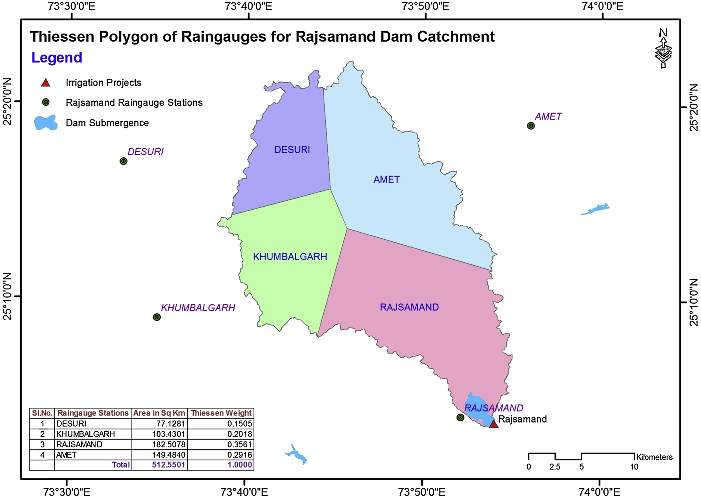
Weighted average rainfall for the catchment is determined using the Thiessen polygon method in this chapter. This method assigns weights to the rain gauges according to the proportions of the total watershed areas that are geographically closest to each of the rain gauges. Weights of individual rain gauges are estimated in proportion to the watershed areas physically associated with the catch of the rain gauge. This method does not account for the orographic influence on the average areal rainfall over the watershed, although this method is most commonly used by the hydrologists due to its simplicity.
A general formula used in the estimation of areal average rainfall of the watershed is given as follows (Eqs. 4.5 and 4.6):
P¯¯¯=∑ni=1wiPi
(4.5)
∑ni=1wi=1
(4.6)
wi=Ai∑iAi=AiA
(4.7)
where P¯¯¯ is the average rainfall, Pi is the rainfall measured at i-th station, n is the number of rain gauges, and wi is the weight assigned to the catch at i-th station. Eq. (4.5) is valid when the condition given by Eq. (4.6) is satisfied. In Eq. (4.7), Ai is the area associated with i-th station or i-th catch, and A is the total area of the watershed.
A methodology for manually constructing the polygons is described by the following steps (Fig. 4.1):
1. Join the exterior most stations by thin lines.
2. Join the inner rain gauges to form well-conditioned triangles.
3. Pick-up a triangle from one side and continue in any direction either clockwise or anticlockwise.
4. Draw the right-angle bisector on the sides of each triangle.
5. Clearly mark the areas between the right-angle bisectors and watershed boundary closely associated with the rain gauges in the form of polygons known as Thiessen polygons.
Figure 4.1 Manual construction of Thiessen polygons.
Table 4.3
Rainfalls Recorded at Four Rain Gauges in the Rajsamand Dam Catchment
Gauge ID
Stations
Monsoon Rainfall (mm)
1
Rajsamand
429.0
2
Amet
298.0
3
Kumbhalgarh
398.0
4
Desuri
436.0
6. Measure the areas of these polygons (Aj) which satisfy the condition given in Eq. (4.6).
7. Determine the Thiessen polygon weights using Eq. (4.7).
8. Estimate the average areal rainfall of the watershed during the particular time using Eq. (4.5).
Example 4.2:
A catchment of Rajsamand irrigation project has a network of seven rain gauges. The monsoon rainfalls (June to September) for the year 2009 recorded at these stations are given in Table 4.3. Calculate the average rainfall over the catchment during Monsoon 2009 using Thiessen polygon method.
Solution:
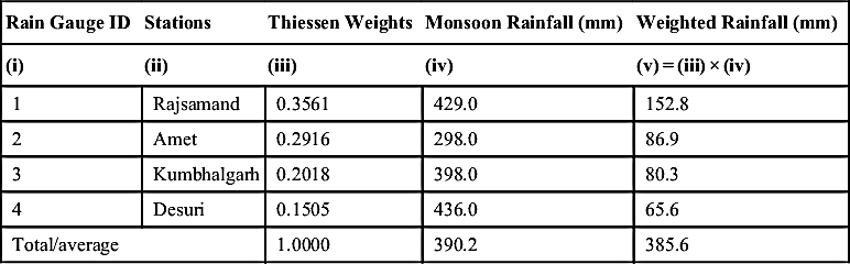
The estimation of the weighted rainfall using the Thiessen polygon method is presented in self-explanatory Table 4.4.
Table 4.4
Estimation of Weighted Average Rainfall Using the Thiessen Polygon Method
Rain Gauge ID
Stations
Thiessen Weights
Monsoon Rainfall (mm)
Weighted Rainfall (mm)
(i)
(ii)
(iii)
(iv)
(v)=(iii)×(iv)
1
Rajsamand
0.3561
429.0
152.8
2
Amet
0.2916
298.0
86.9
3
Kumbhalgarh
0.2018
398.0
80.3
4
Desuri
0.1505
436.0
65.6
Total/average
1.0000
390.2
385.6
4.1.3. Estimation of Rainfall Trends for Climatic Variation: The Mann–Kendall Test
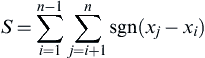
The Mann–Kendall (MK) test searches for a trend in a time series without specifying whether the trend is linear or nonlinear. The Mann–Kendall test for detecting monotonic trends in a hydrologic time series, described by Yue et al. (2002), is based on the test statistics S defined as (Eq. 4.8):
S=∑n−1i=1∑nj=i+1sgn(xj−xi)
(4.8)
where xj are the sequential data values, n is the length of the data set, and
sgn(t)=⎧⎩⎨⎪⎪1,fort>00,fort=0−1,fort<0
(4.9)
The value of S indicates the direction of trend. A negative (positive) value indicates falling (rising) trend. Mann (1945) and Kendall (1955) have documented that when n≥8, the test statistics S is approximately normally distributed with mean and variance as follows (Eqs. 4.10 and 4.11):
E(S)=0
(4.10)
Var(S)=118[n(n−1)(2n+5)−∑mi=1ti(ti−1)(2ti+5)]
(4.11)
where m is the number of tied groups and ti is the size of the i-th tie group. The standardized test statistics Z is computed as follows:
The standardized Mann–Kendall statistics Z follows the standard normal distribution with zero mean and unit variance. If |Z|≥Z1–(α/2), the null hypothesis about no trend is rejected at the significance level α (10% in this study).
An approach to perform a trend analysis of a time series with the presence of significant serial correlation using the Mann–Kendall test is to first remove the serial correlation from the data and then apply the test. Among the various approaches, the prewhitening approach is most common which involves computation of serial correlation and removing the correlation, if the calculated serial correlation is significant at 0.05 significance level. The prewhitening is accomplished as follows:
X′t=xt+1−r1×xt
(4.13)
where xt is the original time series with autocorrelation for time interval t; X′t is the prewhitened time series; and r1 is the lag-1 autocorrelation coefficient. This prewhitened series is then subjected to Mann–Kendall test (i.e., Eqs. 4.8–4.13) for detecting the trend.
Example 4.1 determines the rainfall trend using the Mann–Kendall test for the following weighted rainfalls in the catchment of Meja Dam, Rajasthan.
Year
Annual Rainfall (mm)
Year
Annual Rainfall (mm)
Year
Annual Rainfall (mm)
Year
Annual Rainfall (mm)
1957
491.5
1972
612.0
1987
457.0
2002
137.0
1958
720.3
1973
1011.4
1988
683.3
2003
496.0
1959
317.3
1974
650.9
1989
799.4
2004
832.0
1960
1100.0
1975
819.1
1990
892.7
2005
273.0
1961
830.9
1976
901.4
1991
856.0
2006
821.0
1962
477.7
1977
755.4
1992
796.0
2007
425.0
1963
503.8
1978
764.4
1993
338.1
2008
296.0
1964
492.2
1979
569.0
1994
1051.0
2009
265.0
1965
366.8
1980
354.0
1995
576.4
2010
557.0
1966
750.3
1981
468.7
1996
824.0
2011
558.0
1967
836.7
1982
947.5
1997
925.0
2012
579.0
1968
427.4
1983
900.4
1998
576.0
2013
506.0
1969
585.5
1984
731.2
1999
557.0
1970
868.3
1985
473.1
2000
360.0
1971
591.6
1986
585.4
2001
577.4
Solution:
A computer program has been developed in FORTRAN and used for the computation of the Mann–Kendall test statistics (Appendix A.3). The program generates following outputs:
Lag (k)
Lower Limit
r(k)
Upper Limit
1
−0.236
0.09
0.2
2
−0.238
0.075
0.202
3
−0.24
0.084
0.203
4
−0.243
−0.122
0.205
5
−0.245
0.002
0.207
6
−0.248
0.275
0.208
7
−0.25
0.253
0.21
8
−0.253
−0.061
0.212
9
−0.256
0.084
0.214
10
−0.259
−0.054
0.216
11
−0.262
−0.36
0.218
12
−0.265
0.053
0.22
13
−0.268
−0.022
0.222
14
−0.271
−0.106
0.225
15
−0.275
0.163
0.227
16
−0.278
0.095
0.229
17
−0.282
−0.105
0.232
18
−0.286
−0.073
0.234
19
−0.29
−0.207
0.237
20
−0.294
−0.183
0.24
21
−0.298
0.233
0.243
22
−0.303
0.345
0.245
23
−0.307
0.053
0.249
24
−0.312
0.08
0.252
25
−0.317
−0.276
0.255
26
−0.323
−0.402
0.258
27
−0.329
−0.253
0.262
28
−0.335
0.192
0.266
No. of observations=57;
Value of tie=18;
Var (S)=21,101.0;
Statistic S=−195;
Test statistic Z=−1.33552;
Since absolute value of Z is less than 1.96, there is no trend in data at the 5% significance level.
 (4.1)
(4.1)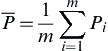 (4.3)
(4.3) (4.4)
(4.4)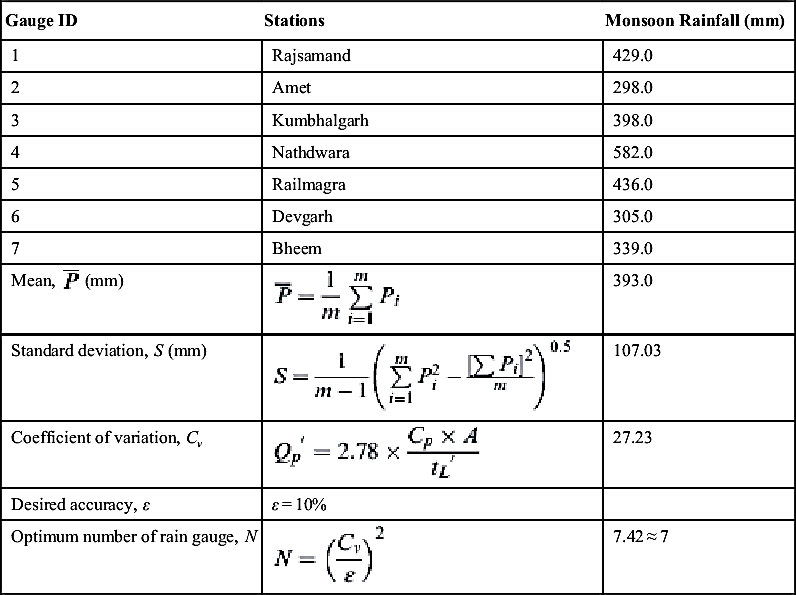
 (4.5)
(4.5) (4.6)
(4.6) (4.7)
(4.7)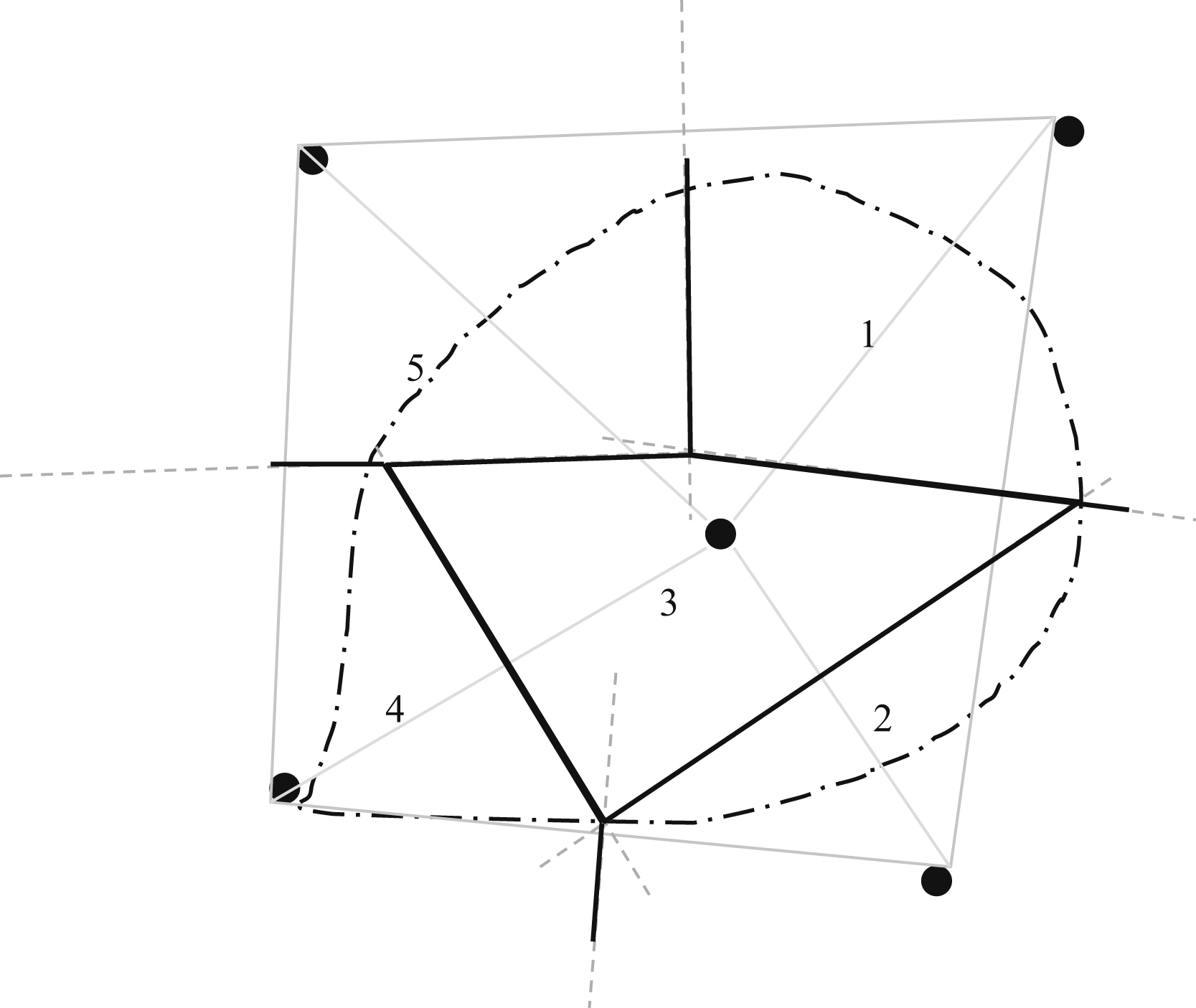
 (4.8)
(4.8) (4.9)
(4.9)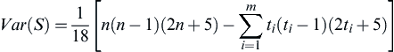 (4.11)
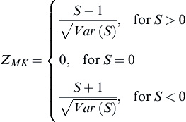 (4.12)
