Search in book...
Toggle Font Controls
Create new playlist

Name your new playlist

Playlist description (optional)
Sign In

Email address

Password

Forgot Password?

or

Continue with Facebook

Continue with Google
Sign Up

Full Name

Email address

Confirm Email Address

Password

or

Continue with Facebook

Continue with Google

Appendices

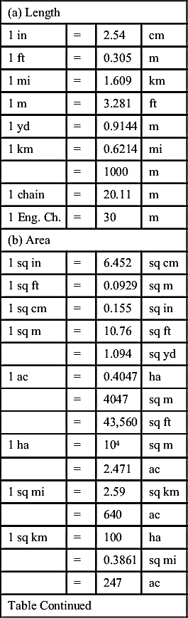
A.1. Unit Conversion Factor

(a) Length
1 in	=	2.54	cm
1 ft	=	0.305	m
1 mi	=	1.609	km
1 m	=	3.281	ft
1 yd	=	0.9144	m
1 km	=	0.6214	mi
	=	1000	m
1 chain	=	20.11	m
1 Eng. Ch.	=	30	m
(b) Area
1 sq in	=	6.452	sq cm
1 sq ft	=	0.0929	sq m
1 sq cm	=	0.155	sq in
1 sq m	=	10.76	sq ft
	=	1.094	sq yd
1 ac	=	0.4047	ha
	=	4047	sq m
	=	43,560	sq ft
1 ha	=	10⁴	sq m
	=	2.471	ac
1 sq mi	=	2.59	sq km
	=	640	ac
1 sq km	=	100	ha
	=	0.3861	sq mi
	=	247	ac
Table Continued

(c) Volume
1 cu ft	=	28.32	L
	=	6.24	imp gal
	=	7.48	US gal
1 Liter (L)	=	1000	cu cm
	=	0.22	imp gal
1 cu m	=	35.3147	cu ft
	=	1000	L
	=	220	gal
1 gal	=	4.546	L
1 ac-ft	=	43,560	cu ft
	=	0.1234	ha-m
	=	1234	cu m
1 cu km	=	0.811	M ac-ft
1 ha-m	=	10⁴	cu m
	=	8.14	ac-ft
	=	0.35315	MCFT
1 M cu m	=	100	ha-m
(1 MCM)	=	10⁶	cu m
	=	814	ac-ft
	=	35.3147	MCFT
(d) Discharge or Flow Rate
1 cusec (cfs)	=	0.02832	m³/s
	=	28.3	lps
	=	1.983	ac-ft/day
	=	374.03	gpm
	=	724	ac-ft/year
1 m³/s	=	35.3147	cusec (cfs)
	=	1000	lps
1 cfs	=	28.3168	lps
Table Continued

1 m³/day	=	2190	imp gpd
1 ac-ft/day	=	1233.5	m³/day
(e) Flow Velocity
1 ft/s	=	30.48	cm/s
1 m/s	=	3.281	ft/s
1 mi/h	=	1.467	ft/s
	=	1.609	km/h
1 knot	=	1.69	ft/s
	=	0.515	m/s
1 km/h	=	1000	m/h
	=	0.2778	m/s
	=	0.9113	ft/s
(f) Mass
1 kg	=	2.205	lb
	=	0.06852	slug
	=	1000	g
	=	10⁶	mg
1 ton	=	1000	kg
1 lb	=	453.6	g
1 slug	=	32.2	lb
	=	14.6	kg
(g) Force (Weight)
1 kgf	=	9.81	N
	=	2.205	lb
1 ln	=	4.448	N
	=	16	oz
(h) Pressure
1 kg/cm³	=	14.23	psi
1 atm	=	14.7	psia
Table Continued

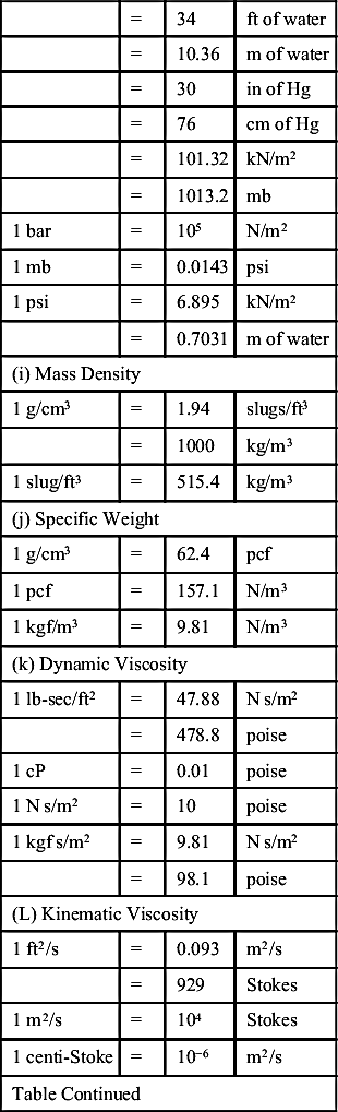
	=	34	ft of water
	=	10.36	m of water
	=	30	in of Hg
	=	76	cm of Hg
	=	101.32	kN/m²
	=	1013.2	mb
1 bar	=	10⁵	N/m²
1 mb	=	0.0143	psi
1 psi	=	6.895	kN/m²
	=	0.7031	m of water
(i) Mass Density
1 g/cm³	=	1.94	slugs/ft³
	=	1000	kg/m³
1 slug/ft³	=	515.4	kg/m³
(j) Specific Weight
1 g/cm³	=	62.4	pcf
1 pcf	=	157.1	N/m³
1 kgf/m³	=	9.81	N/m³
(k) Dynamic Viscosity
1 lb-sec/ft²	=	47.88	N s/m²
	=	478.8	poise
1 cP	=	0.01	poise
1 N s/m²	=	10	poise
1 kgf s/m²	=	9.81	N s/m²
	=	98.1	poise
(L) Kinematic Viscosity
1 ft²/s	=	0.093	m²/s
	=	929	Stokes
1 m²/s	=	10⁴	Stokes
1 centi-Stoke	=	10⁻⁶	m²/s
Table Continued

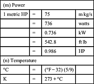
(m) Power
1 metric HP	=	75	m kg/s
	=	736	watts
	=	0.736	kW
	=	542.8	ft lb
	=	0.986	HP
(n) Temperature
°C	=	(°F − 32) (5/9)
K	=	273 + °C

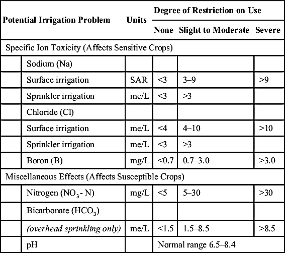
A.2. (A) Guidelines for Interpretations of Water Quality Parameters for Irrigation (¹FAO, 1994)

Potential Irrigation Problem				Units	Degree of Restriction on Use
Potential Irrigation Problem				Units	None	Slight to Moderate	Severe
Salinity (Affects Crop Water Availability)
	EC_w			dS/m	<0.7	0.7–3.0	>3.0
	(or)
	TDS			mg/L	<450	450–2000	>2000
Infiltration (Affects Infiltration Rate of Water Into the Soil. Evaluate Using EC_w and SAR Together)
SAR	=0–3	and EC_w	=		>0.7	0.7–0.2	<0.2
	=3–6		=		>1.2	1.2–0.3	<0.3
	=6–12		=		>1.9	1.9–0.5	<0.5
	=12–20		=		>2.9	2.9–1.3	<1.3
	=20–40		=		>5.0	5.0–2.9	<2.9
Table Continued

Potential Irrigation Problem		Units	Degree of Restriction on Use
Potential Irrigation Problem		Units	None	Slight to Moderate	Severe
Specific Ion Toxicity (Affects Sensitive Crops)
	Sodium (Na)
	Surface irrigation	SAR	<3	3–9	>9
	Sprinkler irrigation	me/L	<3	>3
	Chloride (Cl)
	Surface irrigation	me/L	<4	4–10	>10
	Sprinkler irrigation	me/L	<3	>3
	Boron (B)	mg/L	<0.7	0.7–3.0	>3.0
Miscellaneous Effects (Affects Susceptible Crops)
	Nitrogen (NO₃- N)	mg/L	<5	5–30	>30
	Bicarbonate (HCO₃)
	(overhead sprinkling only)	me/L	<1.5	1.5–8.5	>8.5
	pH		Normal range 6.5–8.4

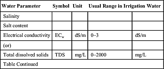
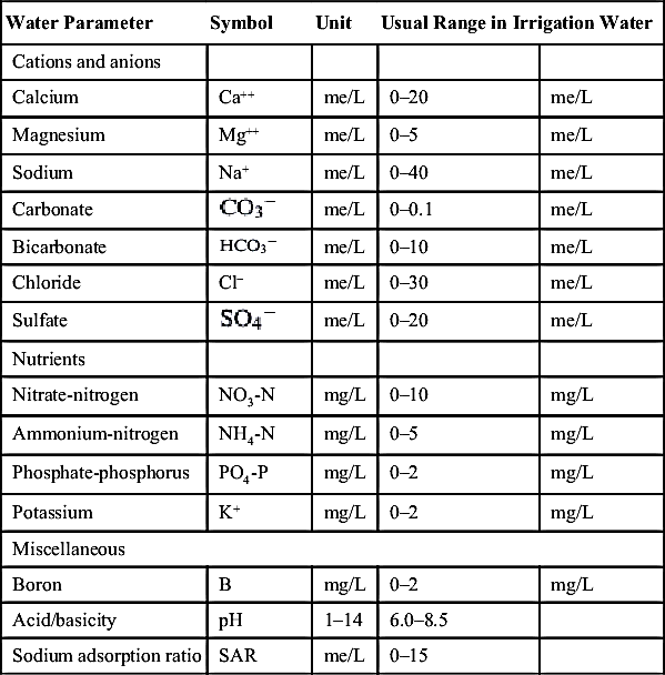
(B) Usual Range of Water Quality Parameters for Irrigation (²FAO, 1994)

Water Parameter	Symbol	Unit	Usual Range in Irrigation Water
Salinity
Salt content
Electrical conductivity	EC_w	dS/m	0–3	dS/m
(or)
Total dissolved solids	TDS	mg/L	0–2000	mg/L
Table Continued

Water Parameter	Symbol	Unit	Usual Range in Irrigation Water
Cations and anions
Calcium	Ca⁺⁺	me/L	0–20	me/L
Magnesium	Mg⁺⁺	me/L	0–5	me/L
Sodium	Na⁺	me/L	0–40	me/L
Carbonate	${CO}_{3}^{-}$ ${CO}_{3}^{-}$	me/L	0–0.1	me/L
Bicarbonate	${HCO}_{3}^{-}$ ${HCO}_{3}^{-}$	me/L	0–10	me/L
Chloride	Cl⁻	me/L	0–30	me/L
Sulfate	${SO}_{4}^{-}$ ${SO}_{4}^{-}$	me/L	0–20	me/L
Nutrients
Nitrate-nitrogen	NO₃-N	mg/L	0–10	mg/L
Ammonium-nitrogen	NH₄-N	mg/L	0–5	mg/L
Phosphate-phosphorus	PO₄-P	mg/L	0–2	mg/L
Potassium	K⁺	mg/L	0–2	mg/L
Miscellaneous
Boron	B	mg/L	0–2	mg/L
Acid/basicity	pH	1–14	6.0–8.5
Sodium adsorption ratio	SAR	me/L	0–15

A.3. FORTRAN Program for Mann–Kendal Test

$DEBUG

C PRGRAMME FOR IDENTIFICATION OF TREND USIN MANN KENDALLS TEST

C WHEN SERIES IS AUTOCORRELETED. IN THIS APPROACH THE TIME SERIES

C IS NORMALIZED USING THE LAG-1 AUTO CORRELATION FUNCTION OF TIME SERIES

DIMENSION X(100,1000),TITLE (80),x1(1000),Y1(1000)

DIMENSION R(50),RKL(50),RKU(50)

OPEN(UNIT=1,FILE=‘Rainfall.IN’,STATUS=‘OLD’)

OPEN(UNIT=2,FILE=‘Surwania_Rainfall_MK_ACF.OUT’)

OPEN(UNIT=3,FILE=‘Surwania_Rainfall_MK_ACF_SUMMARY.OUT’)

READ(1,1)TITLE

1 FORMAT(80A1)

WRITE(2,1)TITLE

C N IS TOTAL NO. OF DATA POINTS IN THE SERIES.

read(1,∗)m,n

c READ(1,∗)N

C X IS THE INPUT SERIES.

do j=1,n

READ(1,∗)(X(I,j),i=1,m)

enddo

do j=1,n

WRITE(2,2)(X(I,j),i=1,m)

enddo

2 FORMAT(1X,(2X,10F7.1))

WRITE(∗,∗)‘SUMMARY OF TREND ANALYSIS USING MANN KENDALL TEST’

WRITE(∗,∗)‘=========================================’

WRITE(∗,∗)

WRITE(∗,∗)‘NO. OF TIME SERIES =’,M

WRITE(∗,∗)‘NO. OF OBSERVATIONS =’,N

WRITE(∗,∗)

WRITE(∗,∗)‘---------------------------------’

WRITE(∗,∗)‘I RKL(1) R(1) RKU(1) ICODE Z COMMENT’

WRITE(∗,∗)‘---------------------------------’

WRITE(3,∗)‘SUMMARY OF TREND ANALYSIS USING MANN KENDALL TEST’

WRITE(3,∗)‘=========================================’

WRITE(3,∗)

WRITE(3,∗)‘NO. OF TIME SERIES =’,M

WRITE(3,∗)‘NO. OF OBSERVATIONS =’,N

WRITE(3,∗)

WRITE(3,∗)‘---------------------------------’

WRITE(3,∗)‘I RKL(1) R(1) RKU(1) ICODE Z COMMENT’

WRITE(3,∗)‘---------------------------------’

do i=1,m

WRITE(2,∗)‘∗∗∗∗∗∗∗∗∗∗∗∗∗∗∗∗∗∗∗∗∗∗∗∗∗∗∗∗∗∗∗∗∗∗∗∗∗∗∗∗∗∗∗∗∗∗∗’

WRITE(2,∗)‘CLIMATIC SERIES=’,I

WRITE(2,∗)‘∗∗∗∗∗∗∗∗∗∗∗∗∗∗∗∗∗∗∗∗∗∗∗∗∗∗∗∗∗∗∗∗∗∗∗∗∗∗∗∗∗∗∗∗∗∗’

do j=1,n

x1(j)=x(i,j)

enddo

CALL ACF(N,X1,R,RKL,RKU)

DO J=1,N-1

Y1(J)=X1(J+1)-R(1)∗X1(J)

ENDDO

IF (R(1).LT.RKL(1).OR.R(1).GT.RKU(1))THEN

ICODE=2 !R1 IS SIGNIFICANT

call mann kendal(n,Y1,ns,vars,z,np,nl,ntie)

IF(ABS(Z).LE.1.96)THEN

ICODE_T=‘NO’

ELSE

ICODE_T=‘YES’

ENDIF

WRITE(∗,4)I,RKL(1),R(1),RKU(1),ICODE,Z,ICODE_T

WRITE(3,4)I,RKL(1),R(1),RKU(1),ICODE,Z,ICODE_T

ELSE

ICODE=1 !R1 IS NOT SIGNIFICANT

CALL MANN KENDAL(N,X1,NS,VARS,Z,NP,NL,NTIE)

IF(ABS(Z).LE.1.96)THEN

ICODE_T=‘NO’

ELSE

ICODE_T=‘YES’

ENDIF

WRITE(∗,4)I,RKL(1),R(1),RKU(1),ICODE,Z,ICODE_T

WRITE(3,4)I,RKL(1),R(1),RKU(1),ICODE,Z,ICODE_T

ENDIF

ENDDO

4 FORMAT(1X,I3,3X,F5.3,2X,F5.3,2X,F5.3,6X,I1,1X,F8.3,3X,A5)

WRITE(∗,∗)‘---------------------------------’

WRITE(3,∗)‘---------------------------------’

stop

end

subroutine mann kendal(n,x,ns,vars,z,np,nl,ntie)

dimension X(1000)

NP=0

NL=0

NTIE=0

DO 51 I=1,N

J=I+1

NT=1

DO 52 I1=J,N

IF(X(I1).GT.X(I))NP=NP+1

IF(X(I1).EQ.X(I))THEN

NT=NT+1

WRITE(2,∗)‘XI=’,X(I1)

ELSE

IF(X(I1).LT.X(I))NL=NL+1

ENDIF

52 CONTINUE

NTIE=NTIE+NT∗(NT-1)∗(2∗NT+5)

51 CONTINUE

NS=(NP-NL)

VARS=(N∗(N-1)∗(2∗N+5)-NTIE)/18

IF(NS.GT.0) THEN

Z=(NS-1)/SQRT(VARS)

ELSEIF(NS.LT.0)THEN

Z=(NS+1)/SQRT(VARS)

ELSE

Z=0

ENDIF

WRITE(2,13)n,NTIE,VARS

13 FORMAT(‘no. of observations=’i4/’ VALUE OF TIE=‘I5/’

1VAR(S)=‘F15.5)

WRITE(2,3)NS,Z

3 FORMAT(‘ VALUE OF S=‘I5/’ TEST STATISTICS=’F10.5)

IF(Z.LT.-1.96)WRITE(2,4)

IF(Z.GE.1.96)WRITE(2,5)

IF(ABS(Z).LT.1.96)WRITE(2,6)

4 FORMAT(‘ THERE IS FALLING TREND IN DATA AT 5% SIGNIFICANCE 1LEVEL’)

5 FORMAT(‘ THERE IS RISING TREND IN DATA AT 5% SIGNIFICANCE 1LEVEL’)

6 FORMAT(‘ THERE IS NO TREND IN DATA AT 5% SIGNIFICANCE LEVEL’)

c write(2,7)(x(i),i=1,n)

7 format(f8.1)

return

END

C PROGRAM TO COMPUTE THE AUTO-CORRELATION FUNCTION

C PROGRAM IS BASED ON THE EQUATION GIVEN BY SALAS ET.AL.(1988)

C PROGRAM WRITTEN BY R.K.RAI

SUBROUTINE ACF(N,X,R,RKL,RKU)

DIMENSION X(500),Y(500),R(50),RKL(50),RKU(50)

K=N/2

WRITE(2,∗)‘--------------------------------’

WRITE(2,∗)‘LAG(K) LOWER LIMIT R(K) UPPER LIMIT’

WRITE(2,∗)‘--------------------------------’

DO KK=1,K

SUMX=0.0

SUMY=0.0

SUMX2=0.0

SUMY2=0.0

SUMXY=0.0

NK=N-KK

DO J=1,N-KK

Y(J)=X(J+KK)

SUMY=SUMY+Y(J)

SUMX=SUMX+X(J)

ENDDO

DO J=1,N-KK

SUMX2=SUMX2+(X(J)-SUMX/NK)∗(X(J)-SUMX/NK)

SUMY2=SUMY2+(Y(J)-SUMY/NK)∗(Y(J)-SUMY/NK)

SUMXY=SUMXY+((X(J)-SUMX/NK)∗(Y(J)-SUMY/NK))

ENDDO

RKL(KK)=(-1-1.645∗SQRT(N-KK-1.))/(N-KK)

R(KK)=SUMXY/(SQRT(SUMX2)∗SQRT(SUMY2))

RKU(KK)=(-1+1.645∗SQRT(N-KK-1.))/(N-KK)

WRITE(2,4)KK,RKL(KK),R(KK),RKU(KK)

ENDDO

4 FORMAT(1X,I3,1X,F8.3,1X,F8.3,1X,F8.3)

WRITE(2,∗)‘--------------------------------’

RETURN

END

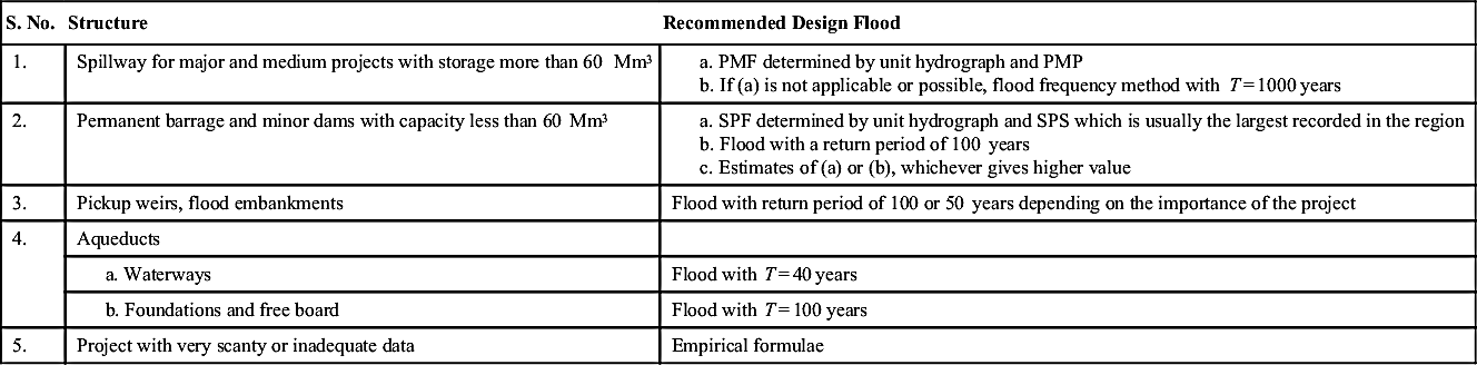
A.4. Guidelines for Selecting the Design Floods (³CBIP, 1989)

S. No.	Structure	Recommended Design Flood
1.	Spillway for major and medium projects with storage more than 60 Mm³	a. PMF determined by unit hydrograph and PMP b. If (a) is not applicable or possible, flood frequency method with T = 1000 years
2.	Permanent barrage and minor dams with capacity less than 60 Mm³	a. SPF determined by unit hydrograph and SPS which is usually the largest recorded in the region b. Flood with a return period of 100 years c. Estimates of (a) or (b), whichever gives higher value
3.	Pickup weirs, flood embankments	Flood with return period of 100 or 50 years depending on the importance of the project
4.	Aqueducts
	a. Waterways	Flood with T = 40 years
	b. Foundations and free board	Flood with T = 100 years
5.	Project with very scanty or inadequate data	Empirical formulae

A.5. Computation of Design Flood for Medium to Small Irrigation Project: Unit Hydrograph Technique

Design of any hydrologic project including irrigation projects, requires estimation of design flood. For estimating the design flood followed by fixing the capacity of the spillway, generally three types of design storms are used: (1) standard project storm (SPS), (2) probable maximum storm or probable maximum precipitation (PMP), and (3) frequency-based storms (FBS).

The SPS is the most severe rainstorm that has actually occurred over a watershed during the period of available records. It is used in the design of all water resources projects where much risk is not involved and economic considerations are taken into account. The SPS is used for design of medium irrigation or water resources projects.

The PMP is defined as the greatest depth of precipitation for a given period which is physically possible over a particular area and geographical location at a certain time of year. PMP is required to estimate the probable maximum flood, used in the design of spillways for large dams including major water resources or irrigation projects. The PMP can be estimated either by statistical methods or by the physical method in which historical rainstorms are maximized. It is generally determined from the greatest rainfall depth associated with severe rainstorm (i.e., SPS).

In FBS, a design flood can be estimated using flood-frequency analysis or frequency analysis of runoff obtained from the maximum rainfall–runoff analysis. The former involves a frequency analysis of long-term streamflow data at a site of interest. The latter involves either the frequency analysis of rainfall followed by rainfall–runoff analysis or frequency analysis of peak runoff estimated from maximum rainfall–peak runoff analysis.

Here, the appendix presents an SPS-based design flood estimation followed by fixing the spillway capacity. The procedure for estimating the design flood is as follows:

1. Determine the most severe rainfall storm (SPS) using the historical data. In India, it can be obtained by a written request to the India Meteorological Department (IMD) for a particular geographical location of interest.

2. Determine the short-term temporal distribution of the SPS: Using the SRRG data, average temporal distribution can be determined, and the same will be used in the determination of temporal distribution of SPS. The same may be requested from the IMD.

3. Determine the rainfall hyetograph (i.e., rainfall intensity vs. time graph and table).

4. Use the constant abstraction rate of the storm (i.e., phi-index), and determine the excess rainfall intensity followed by rainfall excess.

5. Use the derived unit hydrograph (UH) of particular duration for the given catchment.

6. Develop a critical sequence of the rainfall excess using the coordinate of the UH. For arriving at the critical sequences, the following steps are involved:

a. The ordinates of the design UH are written in a column.

b. The highest rainfall excess is written against the peak ordinate of the design UH. The second highest rainfall excess ordinate is written against the second highest ordinate of the UH, which is next to the peak ordinate, and so on. If all the ordinates of UHs are not covered by the rainfall excesses, zeros are put against them.

c. The column of the rainfall excess sequence so generated in step (b) is reversed, i.e., the last value of the rainfall excess is put as the first, the “last but one” is written at the place of the second, and so on. This arrangement of the rainfall excesses is called the “critical sequences.”

7. This critical sequenced rainfall excess is convoluted with design UH to arrive at the design flood.

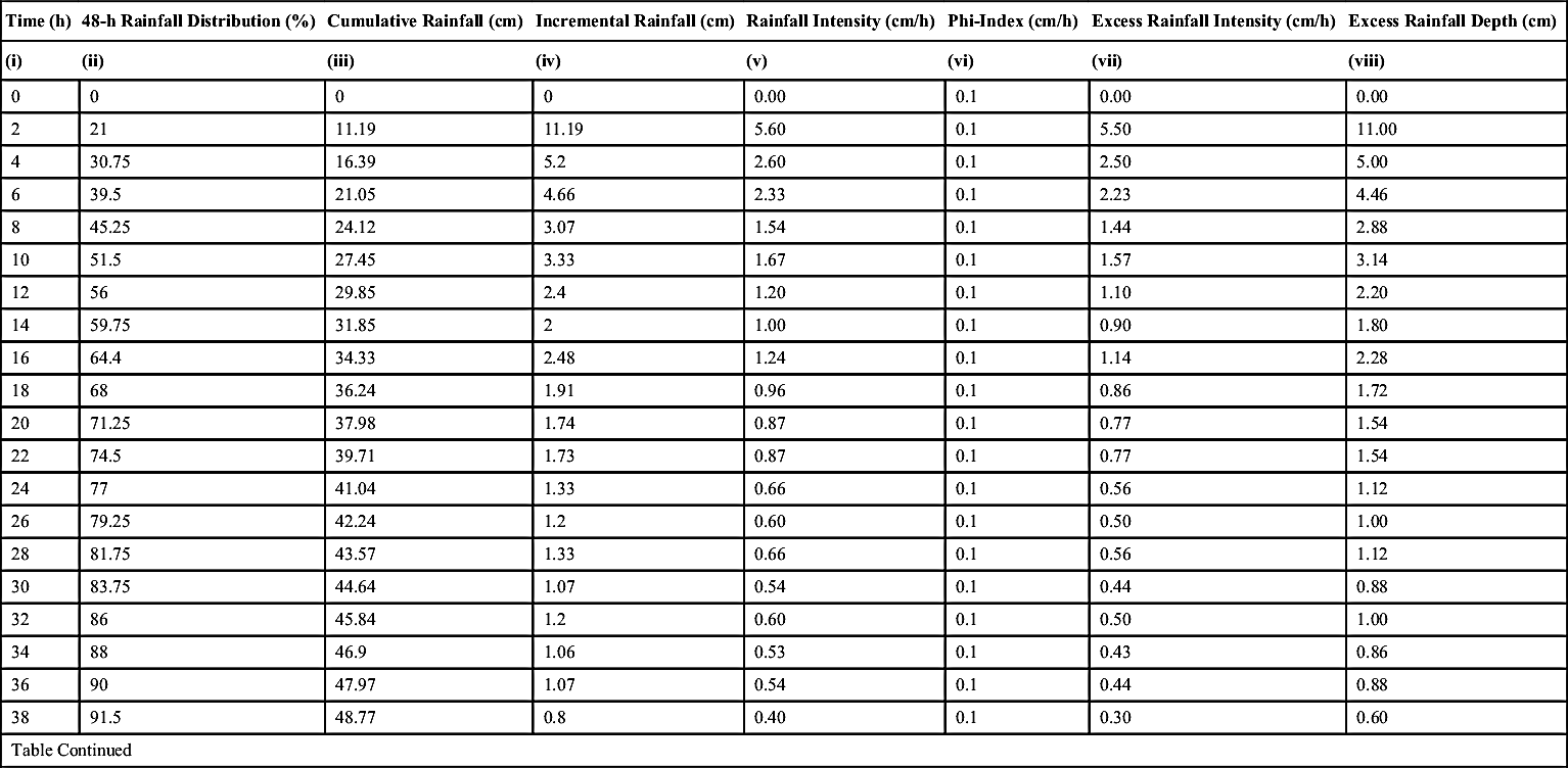
Example A5.1: Estimate the design flood for a medium irrigation project having catchment area of 256 sq km corresponding to the recorded standard project storm (SPS) of 53.3 cm in 48 h. The distribution of rainfall and 2-h UH ordinates are given as under:

Time (h)	0	2	4	6	8	10	12	14	16	18	20	22	24
%Rainfall	0	21.0	30.75	39.5	45.25	51.5	56.0	59.75	64.4	68.0	71.25	74.5	77.0
Time (h)	26	28	30	32	34	36	38	40	42	44	46	48
%Rainfall	79.25	81.75	83.75	86.0	88.0	90.0	91.5	93.5	95.25	97.0	99.0	100.0

Time (h)	0	2	4	6	8	10	12	14	16	18
UH (m³/s/cm)	0	6.69	22.3	83.61	178.73	84.73	33.45	16.17	6	0

Assume phi-index value of 0.10 cm/h and base flow of 34.0 m³/s.

Solution:

(i) Temporal distribution of SPS and excess rainfall estimation

Time (h)	48-h Rainfall Distribution (%)	Cumulative Rainfall (cm)	Incremental Rainfall (cm)	Rainfall Intensity (cm/h)	Phi-Index (cm/h)	Excess Rainfall Intensity (cm/h)	Excess Rainfall Depth (cm)
(i)	(ii)	(iii)	(iv)	(v)	(vi)	(vii)	(viii)
0	0	0	0	0.00	0.1	0.00	0.00
2	21	11.19	11.19	5.60	0.1	5.50	11.00
4	30.75	16.39	5.2	2.60	0.1	2.50	5.00
6	39.5	21.05	4.66	2.33	0.1	2.23	4.46
8	45.25	24.12	3.07	1.54	0.1	1.44	2.88
10	51.5	27.45	3.33	1.67	0.1	1.57	3.14
12	56	29.85	2.4	1.20	0.1	1.10	2.20
14	59.75	31.85	2	1.00	0.1	0.90	1.80
16	64.4	34.33	2.48	1.24	0.1	1.14	2.28
18	68	36.24	1.91	0.96	0.1	0.86	1.72
20	71.25	37.98	1.74	0.87	0.1	0.77	1.54
22	74.5	39.71	1.73	0.87	0.1	0.77	1.54
24	77	41.04	1.33	0.66	0.1	0.56	1.12
26	79.25	42.24	1.2	0.60	0.1	0.50	1.00
28	81.75	43.57	1.33	0.66	0.1	0.56	1.12
30	83.75	44.64	1.07	0.54	0.1	0.44	0.88
32	86	45.84	1.2	0.60	0.1	0.50	1.00
34	88	46.9	1.06	0.53	0.1	0.43	0.86
36	90	47.97	1.07	0.54	0.1	0.44	0.88
38	91.5	48.77	0.8	0.40	0.1	0.30	0.60
Table Continued

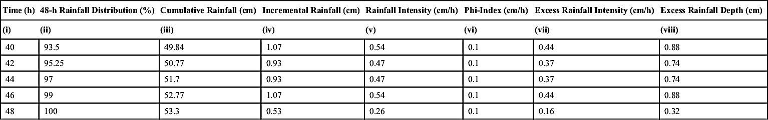
Time (h)	48-h Rainfall Distribution (%)	Cumulative Rainfall (cm)	Incremental Rainfall (cm)	Rainfall Intensity (cm/h)	Phi-Index (cm/h)	Excess Rainfall Intensity (cm/h)	Excess Rainfall Depth (cm)
(i)	(ii)	(iii)	(iv)	(v)	(vi)	(vii)	(viii)
40	93.5	49.84	1.07	0.54	0.1	0.44	0.88
42	95.25	50.77	0.93	0.47	0.1	0.37	0.74
44	97	51.7	0.93	0.47	0.1	0.37	0.74
46	99	52.77	1.07	0.54	0.1	0.44	0.88
48	100	53.3	0.53	0.26	0.1	0.16	0.32

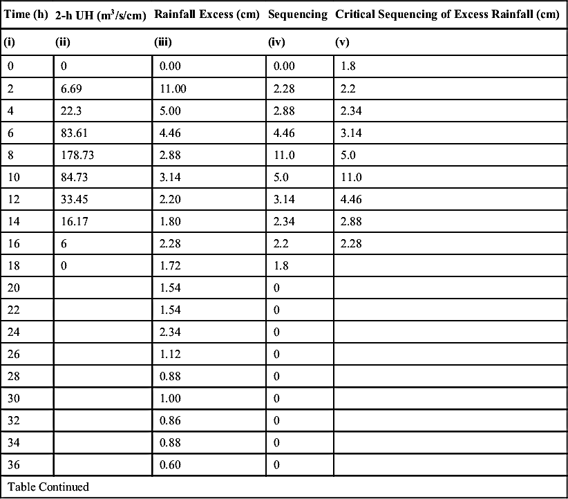
(ii) Critical sequencing of rainfall

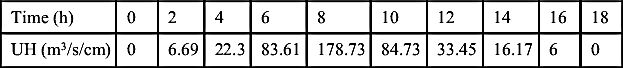
Time (h)	2-h UH (m³/s/cm)	Rainfall Excess (cm)	Sequencing	Critical Sequencing of Excess Rainfall (cm)
(i)	(ii)	(iii)	(iv)	(v)
0	0	0.00	0.00	1.8
2	6.69	11.00	2.28	2.2
4	22.3	5.00	2.88	2.34
6	83.61	4.46	4.46	3.14
8	178.73	2.88	11.0	5.0
10	84.73	3.14	5.0	11.0
12	33.45	2.20	3.14	4.46
14	16.17	1.80	2.34	2.88
16	6	2.28	2.2	2.28
18	0	1.72	1.8
20		1.54	0
22		1.54	0
24		2.34	0
26		1.12	0
28		0.88	0
30		1.00	0
32		0.86	0
34		0.88	0
36		0.60	0
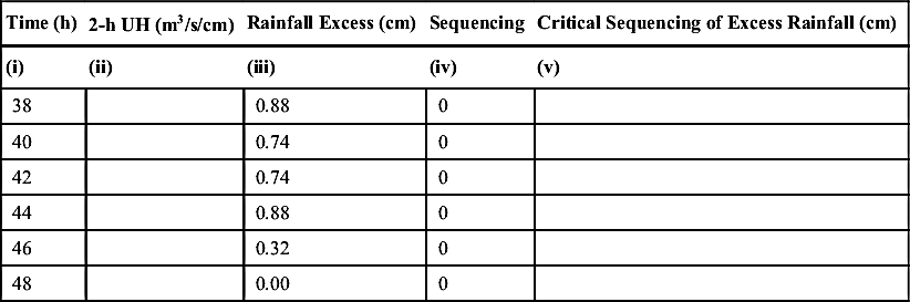
Table Continued

Time (h)	2-h UH (m³/s/cm)	Rainfall Excess (cm)	Sequencing	Critical Sequencing of Excess Rainfall (cm)
(i)	(ii)	(iii)	(iv)	(v)
38		0.88	0
40		0.74	0
42		0.74	0
44		0.88	0
46		0.32	0
48		0.00	0

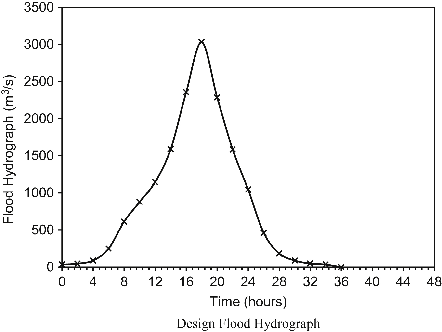
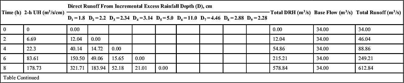
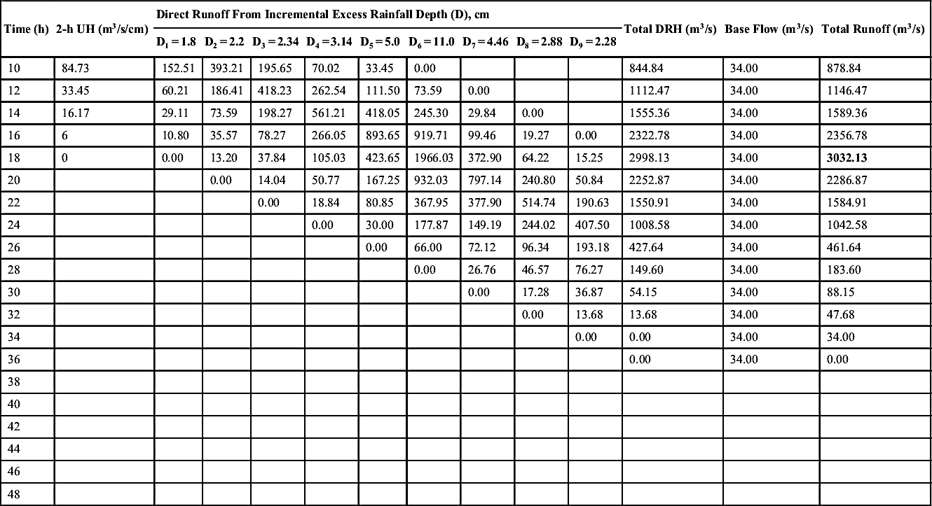
(iii) Determination of design flood hydrograph

Time (h)	2-h UH (m³/s/cm)	Direct Runoff From Incremental Excess Rainfall Depth (D), cm									Total DRH (m³/s)	Base Flow (m³/s)	Total Runoff (m³/s)
Time (h)	2-h UH (m³/s/cm)	D₁ = 1.8	D₂ = 2.2	D₃ = 2.34	D₄ = 3.14	D₅ = 5.0	D₆ = 11.0	D₇ = 4.46	D₈ = 2.88	D₉ = 2.28	Total DRH (m³/s)	Base Flow (m³/s)	Total Runoff (m³/s)
0	0	0.00									0.00	34.00	34.00
2	6.69	12.04	0.00								12.04	34.00	46.04
4	22.3	40.14	14.72	0.00							54.86	34.00	88.86
6	83.61	150.50	49.06	15.65	0.00						215.21	34.00	249.21
8	178.73	321.71	183.94	52.18	21.01	0.00					578.84	34.00	612.84
Table Continued

Time (h)	2-h UH (m³/s/cm)	Direct Runoff From Incremental Excess Rainfall Depth (D), cm									Total DRH (m³/s)	Base Flow (m³/s)	Total Runoff (m³/s)
Time (h)	2-h UH (m³/s/cm)	D₁ = 1.8	D₂ = 2.2	D₃ = 2.34	D₄ = 3.14	D₅ = 5.0	D₆ = 11.0	D₇ = 4.46	D₈ = 2.88	D₉ = 2.28	Total DRH (m³/s)	Base Flow (m³/s)	Total Runoff (m³/s)
10	84.73	152.51	393.21	195.65	70.02	33.45	0.00				844.84	34.00	878.84
12	33.45	60.21	186.41	418.23	262.54	111.50	73.59	0.00			1112.47	34.00	1146.47
14	16.17	29.11	73.59	198.27	561.21	418.05	245.30	29.84	0.00		1555.36	34.00	1589.36
16	6	10.80	35.57	78.27	266.05	893.65	919.71	99.46	19.27	0.00	2322.78	34.00	2356.78
18	0	0.00	13.20	37.84	105.03	423.65	1966.03	372.90	64.22	15.25	2998.13	34.00	3032.13
20			0.00	14.04	50.77	167.25	932.03	797.14	240.80	50.84	2252.87	34.00	2286.87
22				0.00	18.84	80.85	367.95	377.90	514.74	190.63	1550.91	34.00	1584.91
24					0.00	30.00	177.87	149.19	244.02	407.50	1008.58	34.00	1042.58
26						0.00	66.00	72.12	96.34	193.18	427.64	34.00	461.64
28							0.00	26.76	46.57	76.27	149.60	34.00	183.60
30								0.00	17.28	36.87	54.15	34.00	88.15
32									0.00	13.68	13.68	34.00	47.68
34										0.00	0.00	34.00	34.00
36											0.00	34.00	0.00
38
40
42
44
46
48

A.6. Computation of Design Flood for Microirrigation Projects: SCS-CN Method

This method is based on the Soil Conservation Services—Curve Number (SCS-CN) technique (⁴SCS, 1985) through which the designed value of runoff depth is estimated to correspond to design rainfall. The designed rainfall storm corresponds to the daily maximum rainfall of 25–40 years of return period. Once the designed rainfall storm is estimated, the design runoff depth can be computed using the following formula:

$R_{d} = \frac{{(P_{d} - λ S)}^{2}}{P_{d} + (1 - λ) S}$ $R_{d} = \frac{{(P_{d} - λ S)}^{2}}{P_{d} + (1 - λ) S}$

(A6.1)

where R_d is the design value of runoff depth (mm), P_d is the design rainfall depth (mm), S is the maximum potential abstraction (mm), and λ is the abstraction coefficient. The value of λ ranges between 0.1 and 0.3. For black soil, λ = 0.1 for antecedent moisture condition (AMC)-II- and AMC-III-type conditions, and λ = 0.3 for AMC I condition. Since parameter S, i.e., maximum potential abstraction, can vary in the range of 0 ≤ S ≤ ∞, it is mapped onto a dimensionless curve number (CN), varying in a more appealing range 0 ≤ CN ≤ 100, as follows:

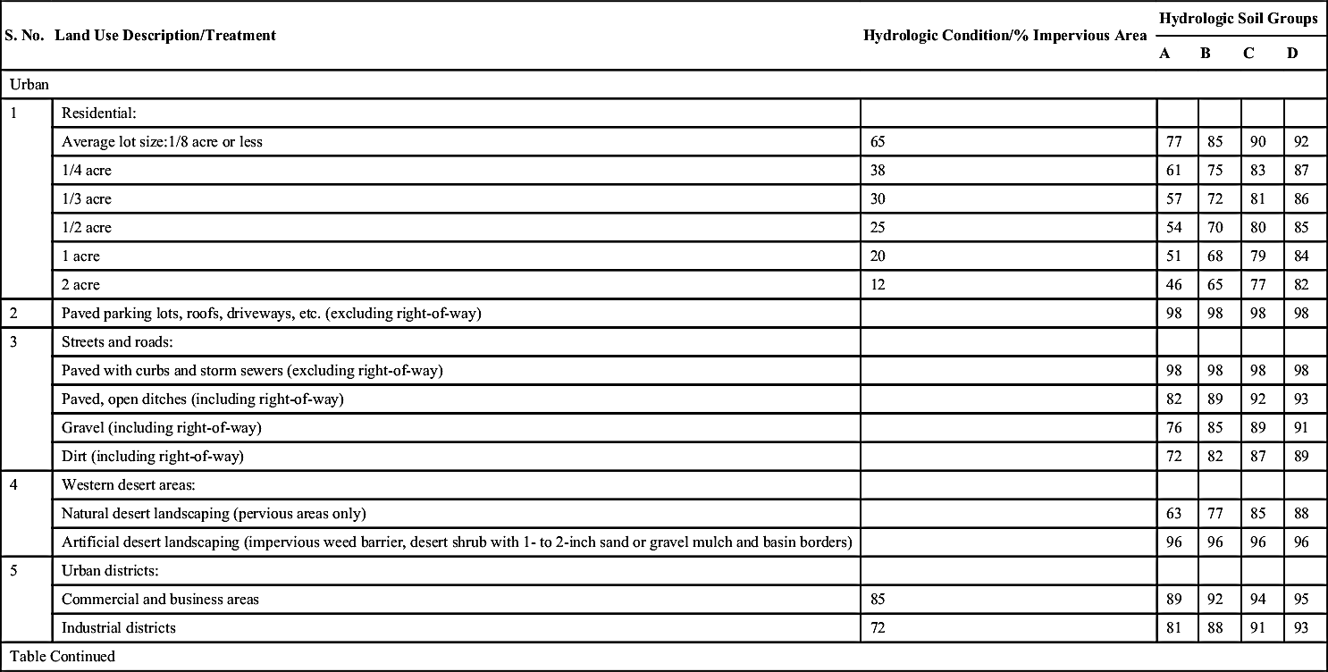
$S = \frac{25400}{C N} - 254$ $S = \frac{25400}{C N} - 254$

(A6.2)

Although CN theoretically varies from 0 to 100, the practical design values validated by experience lie in the range (40, 98). The value of CN tabulated in Appendix A.8 corresponds to the hydrological soil group, AMC condition, and land use.

Once the value of R_d is determined from Eq. (A6.1), the peak discharge or designed discharge can be estimated using the following relationship:

$Q_{p} = 2.08 \times \frac{A \times R_{d}}{t_{p}}$ $Q_{p} = 2.08 \times \frac{A \times R_{d}}{t_{p}}$

(A6.3)

where Q_p is the designed discharge (m³/s), A is the catchment area (sq km), R_d is the design runoff depth (cm), and t_p is the time to peak of the catchment (h).

The value of t_p for small catchment can be determined using the following formula:

$t_{p} = 0.6 t_{c} + t_{c}^{0.5}$ $t_{p} = 0.6 t_{c} + t_{c}^{0.5}$

(A6.4)

where t_p is the time to peak (h) and t_c is the time of concentration (h). The value of t_c can be determined by using the Kirpich formula:

$t_{c} = 0.01947 L^{0.77} S^{- 0.385}$ $t_{c} = 0.01947 L^{0.77} S^{- 0.385}$

(A6.5)

where t_c is in min, L is the length of the channel from headwater to the outlet (m), and S is the slope (m/m).

Another formula for relating the peak discharge rate with the runoff depth and time to peak, generally used in southern India is⁵:

$Q_{p} = 1.46 \times \frac{A \times R_{d}}{t_{p}}$ $Q_{p} = 1.46 \times \frac{A \times R_{d}}{t_{p}}$

(A6.6)

The value of t_p (h) can be determined by using the following relationships:

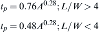$\begin{matrix} t_{p} = 0.76 A^{0.28}; L / W > 4 \\ t_{p} = 0.48 A^{0.28}; L / W < 4 \end{matrix}$ $\begin{matrix} t_{p} = 0.76 A^{0.28}; L / W > 4 \\ t_{p} = 0.48 A^{0.28}; L / W < 4 \end{matrix}$

(A6.7)

where L is the length of the watershed and W is the average width of the watershed (m).

Example A6.1: Estimate the design discharge for a microirrigation project having a catchment area of 25 sq km with a length:width (L:W) ratio of 6. The daily maximum rainfall for 25 years return period is 150 mm. The soil group of the catchment is red soil. The land uses are:

Cultivated land with crops is 60% and waste land is 40%.

Solution:

Catchment area, A = 25 sq km; L:W = 5

Hydrological soil group = red soil (Group B)

(i) The value of t_p can be determined using Eq. (A6.6) as:

$t_{p} = 0.76 A^{0.28} = 0.76 \times 25^{0.28} = 1.87 h$ $t_{p} = 0.76 A^{0.28} = 0.76 \times 25^{0.28} = 1.87 h$

(ii) Computation of CN for hydrological soil group B:

S. No.	Land Uses	%Area	CN	Weighted CN
1	Cultivated land with crops	60.0	75	45
2	Waste land	40.0	80	32
		100	Weighted CN	77

The value of maximum potential abstraction, S will be:

$S = \frac{25400}{C N} - 254 = \frac{25400}{77} - 254 = 75.87 mm$ $S = \frac{25400}{C N} - 254 = \frac{25400}{77} - 254 = 75.87 mm$

(iii) Determined design runoff depth for P_d = 150 mm assuming λ = 0.3

$R_{d} = \frac{{(P_{d} - λ S)}^{2}}{P_{d} + (1 - λ) S} = \frac{{(150 - 0.3 \times 75.87)}^{2}}{150 + 0.7 \times 75.87} = 79.71 mm = 7.97 cm$ $R_{d} = \frac{{(P_{d} - λ S)}^{2}}{P_{d} + (1 - λ) S} = \frac{{(150 - 0.3 \times 75.87)}^{2}}{150 + 0.7 \times 75.87} = 79.71 mm = 7.97 cm$

(iv) Determine the designed discharge using Eq. (A6.3)

$Q_{p} = 2.08 \times \frac{A \times R_{d}}{t_{p}} = 2.08 \times \frac{25 \times 7.97}{1.87} = 221.6 m^{3} / s$ $Q_{p} = 2.08 \times \frac{A \times R_{d}}{t_{p}} = 2.08 \times \frac{25 \times 7.97}{1.87} = 221.6 m^{3} / s$

A.7. Computation of Design Flood: Statistical Distribution Used in Frequency Analysis

There are various statistical distributions, which can be applied in frequency analysis of hydrologic data. The commonly used distribution functions and the best way of use are as follows. The details of these distribution functions can be found in Singh (1998) and Rao and Hamed (2000).

1. Normal Distribution

Normal distribution is used in frequency analysis for fitting empirical distributions to hydrological data, and in simulation of data. As many statistical parameters are approximately normally distributed, the normal distribution is often used for statistical inferences.

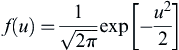
The probability density function:

$f (x) = \frac{1}{σ \sqrt{2 π}} \exp [- \frac{{(x - μ)}^{2}}{2 σ^{2}}]$ $f (x) = \frac{1}{σ \sqrt{2 π}} \exp [- \frac{{(x - μ)}^{2}}{2 σ^{2}}]$

(A7.1)

where μ and σ are the parameters. The standard normal variate u is the normal variable with a mean of 0 and standard deviation equal to 1. Thus the pdf in normal variate form will be:

$f (u) = \frac{1}{\sqrt{2 π}} \exp [- \frac{u^{2}}{2}]$ $f (u) = \frac{1}{\sqrt{2 π}} \exp [- \frac{u^{2}}{2}]$

(A7.2)

where u = (x – μ)/σ. The f(u) function can be numerically estimated using the relation given by Abramowitz and Stegun (1965) as:

$f (u) = (b_{0} + b_{2} u^{2} + b_{4} u^{4} + b_{6} u^{6} + b_{8} u^{8} + b_{10} u^{10}) + ε (u)$ $f (u) = (b_{0} + b_{2} u^{2} + b_{4} u^{4} + b_{6} u^{6} + b_{8} u^{8} + b_{10} u^{10}) + ε (u)$

(A7.3)

where

$\begin{matrix} \begin{matrix} b_{0} = 2.5052367 \\ b_{2} = 1.2831204 \\ b_{4} = 0.2264718 \end{matrix} & \begin{matrix} b_{6} = 0.1306469 \\ b_{8} = - 0.020249 \\ b_{10} = 0.0039132 \end{matrix} \end{matrix}$ $\begin{matrix} \begin{matrix} b_{0} = 2.5052367 \\ b_{2} = 1.2831204 \\ b_{4} = 0.2264718 \end{matrix} & \begin{matrix} b_{6} = 0.1306469 \\ b_{8} = - 0.020249 \\ b_{10} = 0.0039132 \end{matrix} \end{matrix}$

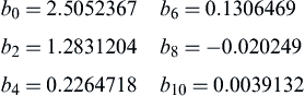(A7.4)

The cumulative distribution of normal variate is given by:

$F (u) = \int_{- \infty}^{u} \frac{1}{\sqrt{2 π}} \exp (- t^{2} / 2) d t$ $F (u) = \int_{- \infty}^{u} \frac{1}{\sqrt{2 π}} \exp (- t^{2} / 2) d t$

(A7.5)

A numerical approximation of Eq. (A7.5) given by Abramowitz and Stegun (1965) is:

$F (u) = 1 - f (u) (b_{1} q + b_{2} q^{2} + b_{3} q^{3} + b_{4} q^{4} + b_{5} q^{5}) + ε (u)$ $F (u) = 1 - f (u) (b_{1} q + b_{2} q^{2} + b_{3} q^{3} + b_{4} q^{4} + b_{5} q^{5}) + ε (u)$

(A7.6)

where

$q = \frac{1}{1 + p u}, p = 0.2316419 and 0 \leq u < \infty$ $q = \frac{1}{1 + p u}, p = 0.2316419 and 0 \leq u < \infty$

(A7.7)

$\begin{matrix} \begin{matrix} b_{1} = 0.319381530 \\ b_{2} = - 0.356563782 \\ b_{3} = 1.781477937 \end{matrix} & \begin{matrix} b_{4} = - 1.821255978 \\ b_{5} = 1.330274429 \end{matrix} \end{matrix}$ $\begin{matrix} \begin{matrix} b_{1} = 0.319381530 \\ b_{2} = - 0.356563782 \\ b_{3} = 1.781477937 \end{matrix} & \begin{matrix} b_{4} = - 1.821255978 \\ b_{5} = 1.330274429 \end{matrix} \end{matrix}$

(A7.8)

$F (- u) = 1 - F (u)$ $F (- u) = 1 - F (u)$

(A7.9)

Parameter estimation:

$Method of moments (MoM): \hat{μ} = m_{1}^{'}; \hat{σ} = \sqrt{m_{2}}$ $Method of moments (MoM): \hat{μ} = m_{1}^{'}; \hat{σ} = \sqrt{m_{2}}$

(A7.10a,b)

$Probability weighted moments (PWM): \hat{μ} = l_{1}; \hat{σ} = \sqrt{π} l_{2}$ $Probability weighted moments (PWM): \hat{μ} = l_{1}; \hat{σ} = \sqrt{π} l_{2}$

(A7.11a,b)

Quantile estimate:

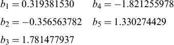
For a given return period T, the corresponding probability of nonexceedance is F = 1 − 1/T. It is easy to calculate the standard normal variate u corresponding to a probability F of nonexceedence. Abramowitz and Stegun (1965) gave the value of u corresponding to the probability of exceedence P as follows:

$u = W - \frac{c_{0} + c_{1} W + c_{2} W^{2}}{1 + d_{1} W + d_{2} W^{2} + d_{3} W^{3}}$ $u = W - \frac{c_{0} + c_{1} W + c_{2} W^{2}}{1 + d_{1} W + d_{2} W^{2} + d_{3} W^{3}}$

(A7.12)

where

$W = \sqrt{- 2 \ln (P)} for P < 0.5 and P = 1 - F$ $W = \sqrt{- 2 \ln (P)} for P < 0.5 and P = 1 - F$

(A7.13a)

$For P > 0.5, W = \sqrt{- 2 \ln (1 - P)}$ $For P > 0.5, W = \sqrt{- 2 \ln (1 - P)}$

(A7.13b)

and

$\begin{matrix} \begin{matrix} c_{0} = 2.515517 \\ c_{1} = 0.802853 \\ c_{2} = 0.010328 \end{matrix} & \begin{matrix} d_{1} = 1.432788 \\ d_{2} = 0.189269 \\ d_{3} = 0.001308 \end{matrix} \end{matrix}$ $\begin{matrix} \begin{matrix} c_{0} = 2.515517 \\ c_{1} = 0.802853 \\ c_{2} = 0.010328 \end{matrix} & \begin{matrix} d_{1} = 1.432788 \\ d_{2} = 0.189269 \\ d_{3} = 0.001308 \end{matrix} \end{matrix}$

(A7.14)

When P > .5, the required value of u is taken as opposite sign of the estimated value.

Chow (1964) proposed the following general form of the quantile estimate formula:

${\hat{x}}_{T} = μ_{1} + K_{T} \sqrt{μ_{2}}$ ${\hat{x}}_{T} = μ_{1} + K_{T} \sqrt{μ_{2}}$

(A7.15)

where K_T is the frequency factor, which is a function of the return period and the parameters of the distribution. For normal distribution, the required quantile estimate is calculated using the following relationship:

${\hat{x}}_{T} = \hat{μ} + \hat{σ} u$ ${\hat{x}}_{T} = \hat{μ} + \hat{σ} u$

(A7.16)

Standard error of estimate

$MoM: S_{T} = {[1 + \frac{u^{2}}{2}]}^{1 / 2} \cdot \frac{σ}{\sqrt{n}}$ $MoM: S_{T} = {[1 + \frac{u^{2}}{2}]}^{1 / 2} \cdot \frac{σ}{\sqrt{n}}$

(A7.17)

$PWM: S_{T} = {[1 + 0.5113 u^{2}]}^{1 / 2} \frac{\hat{σ}}{\sqrt{n}}$ $PWM: S_{T} = {[1 + 0.5113 u^{2}]}^{1 / 2} \frac{\hat{σ}}{\sqrt{n}}$

(A7.18)

Confidence interval:

An approximate (1 − α) confidence interval for

{\hat{x}}_{T}

${\hat{x}}_{T}$

is given by:

$\frac{l}{u} = {\hat{x}}_{T} \mp Z_{α / 2} S_{T}$ $\frac{l}{u} = {\hat{x}}_{T} \mp Z_{α / 2} S_{T}$

(A7.19)

where α is the significance level. For 5% significance level (i.e., 95% confidence level) Z_α/2 = 1.96. For 90% and 99% confidence interval, the values of Z_α/2 are 1.645 and 2.575, respectively.

2. Log-Normal Distribution

Parameters of the log-normal distribution using MoM and PWM are estimated, and are related to their sample moments and L-moments as follows:

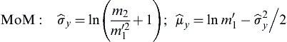$MoM: {\hat{σ}}_{y} = \ln (\frac{m_{2}}{m_{1}^{' 2}} + 1); {\hat{μ}}_{y} = \ln m_{1}^{'} - {\hat{σ}}_{y}^{2} / 2$ $MoM: {\hat{σ}}_{y} = \ln (\frac{m_{2}}{m_{1}^{' 2}} + 1); {\hat{μ}}_{y} = \ln m_{1}^{'} - {\hat{σ}}_{y}^{2} / 2$

(A7.20a,b)

$PWM: {\hat{σ}}_{y} = 2 {erf}^{- 1} (t); {\hat{μ}}_{y} = \ln l_{1} - {\hat{σ}}_{y}^{2} / 2$ $PWM: {\hat{σ}}_{y} = 2 {erf}^{- 1} (t); {\hat{μ}}_{y} = \ln l_{1} - {\hat{σ}}_{y}^{2} / 2$

(A7.21a,b)

where

${erf}^{- 1} (x) = \frac{2}{\sqrt{π}} \int_{0}^{x} \exp (- u^{2}) d u = 2 F (x / \sqrt{2}) - 1$ ${erf}^{- 1} (x) = \frac{2}{\sqrt{π}} \int_{0}^{x} \exp (- u^{2}) d u = 2 F (x / \sqrt{2}) - 1$

(A7.22)

Quantile estimates: The flood quantile is estimated using the following relationship:

${\hat{x}}_{T} = \exp [{\hat{μ}}_{y} + u {\hat{σ}}_{y}]$ ${\hat{x}}_{T} = \exp [{\hat{μ}}_{y} + u {\hat{σ}}_{y}]$

(A7.23)

In the form of frequency factor, Eq. (A7.23) can be written as follows:

${\hat{x}}_{T} = \exp [\hat{μ} + K_{T} \hat{σ}]$ ${\hat{x}}_{T} = \exp [\hat{μ} + K_{T} \hat{σ}]$

(A7.24)

with

$K_{T} = \frac{\exp [{\hat{σ}}_{y}^{u} - {\hat{σ}}_{y}^{2} / 2] - 1}{{[\exp ({\hat{σ}}_{y}^{2}) - 1]}^{1 / 2}}$ $K_{T} = \frac{\exp [{\hat{σ}}_{y}^{u} - {\hat{σ}}_{y}^{2} / 2] - 1}{{[\exp ({\hat{σ}}_{y}^{2}) - 1]}^{1 / 2}}$

(A7.25)

where

\hat{μ}

$\hat{μ}$

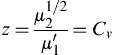
and

\hat{σ}

$\hat{σ}$

are the mean and standard deviation of the original series.

Standard error:

The standard error while using the MoM as parameter estimator is estimated using the following expression:

$S_{T} = δ_{y} \frac{\hat{σ}}{\sqrt{n}}$ $S_{T} = δ_{y} \frac{\hat{σ}}{\sqrt{n}}$

(A7.26)

with

$δ_{y} = {[1 + (z^{3} + 3 z) K_{T} + (z^{8} + 6 z^{6} + 15 z^{4} + 16 z^{2} + 2) K_{T}^{2} / 4]}^{1 / 2}$ $δ_{y} = {[1 + (z^{3} + 3 z) K_{T} + (z^{8} + 6 z^{6} + 15 z^{4} + 16 z^{2} + 2) K_{T}^{2} / 4]}^{1 / 2}$

(A7.27a)

and

$z = \frac{μ_{2}^{1 / 2}}{μ_{1}^{'}} = C_{v}$ $z = \frac{μ_{2}^{1 / 2}}{μ_{1}^{'}} = C_{v}$

(A7.27b)

3. Two-Parameter Gamma Distribution

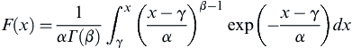
It is a widely used distribution function in hydrology. In many cases, event-based hydrographs, monthly rainfall, etc., follow gamma distribution. The pdf and cdf of the gamma distribution are expressed as follows:

$f (x) = \frac{1}{α^{β} Γ (β)} x^{β - 1} \exp (- x / α)$ $f (x) = \frac{1}{α^{β} Γ (β)} x^{β - 1} \exp (- x / α)$

(A7.28)

$F (x) = \frac{1}{α^{β} Γ (β)} \int_{0}^{x} x^{β - 1} \exp (- x / α) d x$ $F (x) = \frac{1}{α^{β} Γ (β)} \int_{0}^{x} x^{β - 1} \exp (- x / α) d x$

(A7.29)

Substituting

y = x / α

$y = x / α$

, we get the following form of the cdf:

$F (y) = \frac{1}{Γ (β)} \int_{0}^{y} y^{β - 1} \exp (- y) d y$ $F (y) = \frac{1}{Γ (β)} \int_{0}^{y} y^{β - 1} \exp (- y) d y$

(A7.30)

Parameter estimation:

$MoM: \hat{α} = \frac{m_{2}}{m_{1}^{'}}$ $MoM: \hat{α} = \frac{m_{2}}{m_{1}^{'}}$

(A7.31)

with

$m_{2} = {(C_{v} m_{1}^{'})}^{2}$ $m_{2} = {(C_{v} m_{1}^{'})}^{2}$

(A7.32)

$\hat{β} = \frac{{(m_{1}^{'})}^{2}}{m_{2}}$ $\hat{β} = \frac{{(m_{1}^{'})}^{2}}{m_{2}}$

(A7.33)

The skewness coefficient is given by:

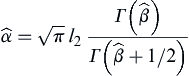
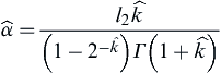
$C_{s} = \frac{α}{| α |} \frac{2}{\sqrt{β}}$ $C_{s} = \frac{α}{| α |} \frac{2}{\sqrt{β}}$

(A7.34)

PWM: Hosking (1990) gave the following relationships for estimating the parameters α and β using the probability weighted moments.

If 0 < t < ½, where t = l₂/l₁, then z = πt² and

$\hat{β} = \frac{1 - 0.3080 z}{z - 0.05812 z^{2} + 0.01765 z^{3}}$ $\hat{β} = \frac{1 - 0.3080 z}{z - 0.05812 z^{2} + 0.01765 z^{3}}$

(A7.35)

\frac{1}{2} \leq t < 1

$\frac{1}{2} \leq t < 1$

then z = 1 − t and

$\hat{β} = \frac{0.7213 z - 0.5947 z^{2}}{1 - 2.1817 z + 1.2113 z^{2}}$ $\hat{β} = \frac{0.7213 z - 0.5947 z^{2}}{1 - 2.1817 z + 1.2113 z^{2}}$

(A7.36)

$\hat{α} = l_{1} / \hat{β}$ $\hat{α} = l_{1} / \hat{β}$

(A7.37)

Quantile estimates: Kite (1977) shows that the frequency factor K_T for the two-parameter gamma distribution is:

$K_{T} = \frac{χ^{2} C_{s}}{4} - \frac{2}{C_{s}}$ $K_{T} = \frac{χ^{2} C_{s}}{4} - \frac{2}{C_{s}}$

(A7.38)

where

C_{s} = \frac{m_{3}}{m_{2}^{3 / 2}}

$C_{s} = \frac{m_{3}}{m_{2}^{3 / 2}}$

and χ² can be obtained using the following relation:

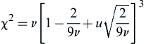$χ^{2} = ν {[1 - \frac{2}{9 ν} + u \sqrt{\frac{2}{9 ν}}]}^{3}$ $χ^{2} = ν {[1 - \frac{2}{9 ν} + u \sqrt{\frac{2}{9 ν}}]}^{3}$

(A7.39)

where u is the standard normal variate corresponding to a probability of nonexceedance of

F = 1 - 1 / T

$F = 1 - 1 / T$

; ν is the degree of freedom = 2β. Several expressions for estimating K_T directly from C_s are suggested by Bobée and Ashkar (1991). The approximation suggested by Wilson and Hilferty (1931), known as Wilson–Hilferty transformation, can be used, which is expressed as follows:

For C_s ≤ 1.0 up to C_s = 2:

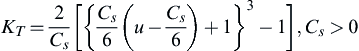$K_{T} = \frac{2}{C_{s}} [{\frac{C_{s}}{6} (u - \frac{C_{s}}{6}) + 1}^{3} - 1], C_{s} > 0$ $K_{T} = \frac{2}{C_{s}} [{\frac{C_{s}}{6} (u - \frac{C_{s}}{6}) + 1}^{3} - 1], C_{s} > 0$

(A7.40)

The T-year quantile is then estimated using the following expression:

${\hat{x}}_{T} = \hat{α} \hat{β} + K_{T} \sqrt{{\hat{α}}^{2} \hat{β}}$ ${\hat{x}}_{T} = \hat{α} \hat{β} + K_{T} \sqrt{{\hat{α}}^{2} \hat{β}}$

(A7.41)

Standard error: While using the MoM for parameter estimation the standard error of estimate in the quantile can be estimated using the following formula:

$S_{T}^{2} = \frac{m_{2}}{n} [{(1 + K_{T} C_{v})}^{2} + \frac{1}{2} {(K_{T} + 2 C_{v} \frac{\partial K_{T}}{\partial C_{s}})}^{2} (1 + C_{v}^{2})]$ $S_{T}^{2} = \frac{m_{2}}{n} [{(1 + K_{T} C_{v})}^{2} + \frac{1}{2} {(K_{T} + 2 C_{v} \frac{\partial K_{T}}{\partial C_{s}})}^{2} (1 + C_{v}^{2})]$

(A7.42)

where C_v is the coefficient of variation and K_T is the frequency factor. The term

\frac{\partial K_{T}}{\partial C_{s}}

$\frac{\partial K_{T}}{\partial C_{s}}$

is calculated from the Wilson–Hilferty transformation formula for K_T by taking the partial differentiation with respect to C_s and is given as follows:

$\frac{\partial K_{T}}{\partial C_{s}} = \frac{- 2}{C_{s}^{2}} [{\frac{C_{s}}{6} (u - \frac{C_{s}}{6}) + 1}^{3} + 1] + \frac{2}{C_{s}} [3 {\frac{C_{s}}{6} (u - \frac{C_{s}}{6}) + 1}^{2} (\frac{u}{6} - \frac{2 C_{s}}{36})]$ $\frac{\partial K_{T}}{\partial C_{s}} = \frac{- 2}{C_{s}^{2}} [{\frac{C_{s}}{6} (u - \frac{C_{s}}{6}) + 1}^{3} + 1] + \frac{2}{C_{s}} [3 {\frac{C_{s}}{6} (u - \frac{C_{s}}{6}) + 1}^{2} (\frac{u}{6} - \frac{2 C_{s}}{36})]$

(A7.43)

The confidence interval can be calculated similar to the normal distribution.

4. Pearson (3) Distribution

The pdf and cdf of the Pearson (3) distribution are given by:

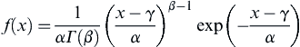$f (x) = \frac{1}{α Γ (β)} {(\frac{x - γ}{α})}^{β - 1} \exp (- \frac{x - γ}{α})$ $f (x) = \frac{1}{α Γ (β)} {(\frac{x - γ}{α})}^{β - 1} \exp (- \frac{x - γ}{α})$

(A7.44)

where

$Γ (y + 1) = \int_{0}^{\infty} t^{y} \exp (- t) d t; y + 1 > 0$ $Γ (y + 1) = \int_{0}^{\infty} t^{y} \exp (- t) d t; y + 1 > 0$

(A7.45)

$Γ (n + 1) = n!; n is positive integer$ $Γ (n + 1) = n!; n is positive integer$

(A7.46)

The cdf is:

$F (x) = \frac{1}{α Γ (β)} \int_{γ}^{x} {(\frac{x - γ}{α})}^{β - 1} \exp (- \frac{x - γ}{α}) d x$ $F (x) = \frac{1}{α Γ (β)} \int_{γ}^{x} {(\frac{x - γ}{α})}^{β - 1} \exp (- \frac{x - γ}{α}) d x$

(A7.47)

y = (x - γ) / α

$y = (x - γ) / α$

then

$F (y) = \frac{1}{Γ (β)} \int_{γ}^{(x - γ) / α} y^{β - 1} \exp (- y) d y$ $F (y) = \frac{1}{Γ (β)} \int_{γ}^{(x - γ) / α} y^{β - 1} \exp (- y) d y$

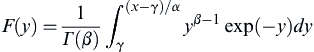(A7.48)

Parameter estimation

$MoM: \hat{β} = {(2 / C_{s})}^{2}$ $MoM: \hat{β} = {(2 / C_{s})}^{2}$

(A7.49)

$\hat{α} = \sqrt{m_{2} / \hat{β}}$ $\hat{α} = \sqrt{m_{2} / \hat{β}}$

(A7.50)

$\hat{γ} = m_{1}^{'} - \sqrt{m_{2} \hat{β}}$ $\hat{γ} = m_{1}^{'} - \sqrt{m_{2} \hat{β}}$

(A7.51)

PWM: For t₃ > 1/3, let t_m = 1 − t₃ then

$\hat{β} = \frac{0.36067 t_{m} - 0.5967 t_{m}^{2} + 0.025361 t_{m}^{3}}{1 - 2.78861 t_{m} + 2.56096 t_{m}^{2} - 0.77045 t_{m}^{3}}$ $\hat{β} = \frac{0.36067 t_{m} - 0.5967 t_{m}^{2} + 0.025361 t_{m}^{3}}{1 - 2.78861 t_{m} + 2.56096 t_{m}^{2} - 0.77045 t_{m}^{3}}$

(A7.52)

For t₃ < 1/3, let

t_{m} = 3 π t_{3}^{2}

$t_{m} = 3 π t_{3}^{2}$

then

$\hat{β} = \frac{1 + 0.2906 t_{m}}{t_{m} + 0.1882 t_{m}^{2} + 0.0442 t_{m}^{3}}$ $\hat{β} = \frac{1 + 0.2906 t_{m}}{t_{m} + 0.1882 t_{m}^{2} + 0.0442 t_{m}^{3}}$

(A7.53)

$\hat{α} = \sqrt{π} l_{2} \frac{Γ (\hat{β})}{Γ (\hat{β} + 1 / 2)}$ $\hat{α} = \sqrt{π} l_{2} \frac{Γ (\hat{β})}{Γ (\hat{β} + 1 / 2)}$

(A7.54)

$\hat{γ} = l_{1} - \hat{α} \hat{β}$ $\hat{γ} = l_{1} - \hat{α} \hat{β}$

(A7.55)

Quantile estimate:

The flood quantile is estimated using the following formula:

${\hat{x}}_{T} = \hat{α} \hat{β} + \hat{γ} + K_{T} \sqrt{{\hat{α}}^{2} \hat{β}}$ ${\hat{x}}_{T} = \hat{α} \hat{β} + \hat{γ} + K_{T} \sqrt{{\hat{α}}^{2} \hat{β}}$

(A7.56)

where K_T is the frequency factor corresponding to a return period of T years and can be calculated using the steps similar to those involved in the gamma distribution.

Standard error: While using the MoM for parameter estimation the standard error of estimate in the quantile can be estimated using the following formula:

$S_{T}^{2} = \frac{m_{2}}{n} [1 + K_{T} C_{s} + \frac{K_{T}^{2}}{2} (\frac{3 C_{s}^{2}}{4} + 1) + 3 K_{T} \frac{\partial K_{T}}{\partial C_{s}} (C_{s} + \frac{C_{s}^{3}}{4}) + 3 {(\frac{\partial K_{T}}{\partial C_{s}})}^{2} (2 + 3 C_{s}^{2} + \frac{5 C_{s}^{4}}{8})]$ $S_{T}^{2} = \frac{m_{2}}{n} [1 + K_{T} C_{s} + \frac{K_{T}^{2}}{2} (\frac{3 C_{s}^{2}}{4} + 1) + 3 K_{T} \frac{\partial K_{T}}{\partial C_{s}} (C_{s} + \frac{C_{s}^{3}}{4}) + 3 {(\frac{\partial K_{T}}{\partial C_{s}})}^{2} (2 + 3 C_{s}^{2} + \frac{5 C_{s}^{4}}{8})]$

(A7.57)

5. Log-Pearson (3) Distribution

The easy way of fitting the log-Pearson [LP (3)] distribution is to take the logarithm of the variable and follow the similar steps mentioned in case of Pearson (3) distribution. The flood quantile is estimated using the following expression:

${\hat{x}}_{T} = \exp ({\hat{y}}_{T})$ ${\hat{x}}_{T} = \exp ({\hat{y}}_{T})$

(A7.58)

where y = ln x.

The LP (3) distribution is also recommended by the US Water Resources Council for flood-frequency analysis related to federal projects (USWRC, 1967, 1976, 1977, 1981).

6. Extreme Value Type I Distribution (Gumbel Distribution)

The extreme value type I is most commonly used distribution function applied in flood-frequency analysis of annual maximum flow series. It is also known as the Gumbel distribution. The pdf and cdf of this distribution are expressed by Eqs. (A7.59) and (A7.60), respectively.

$f (x) = \frac{1}{α} \exp [- (\frac{x - β}{α}) - \exp (- \frac{x - β}{α})]; - \infty < x < \infty$ $f (x) = \frac{1}{α} \exp [- (\frac{x - β}{α}) - \exp (- \frac{x - β}{α})]; - \infty < x < \infty$

(A7.59)

$F (x) = \exp [- \exp (- \frac{x - β}{α})]$ $F (x) = \exp [- \exp (- \frac{x - β}{α})]$

(A7.60)

Parameter estimation: Parameters α and β are related with sample moments and L-moments ratios in case of MoM and PWM methods, respectively.

MoM:

$\hat{α} = \frac{\sqrt{6}}{π} \sqrt{m_{2}} = 0.7797 \sqrt{m_{2}}$ $\hat{α} = \frac{\sqrt{6}}{π} \sqrt{m_{2}} = 0.7797 \sqrt{m_{2}}$

(A7.61)

$\hat{β} = m_{1}^{'} - 0.45005 \sqrt{m_{2}}$ $\hat{β} = m_{1}^{'} - 0.45005 \sqrt{m_{2}}$

(A7.62)

PWM:

$\hat{α} = (2 b_{1} - b_{0}) / \ln 2 = \frac{l_{2}}{\ln 2}$ $\hat{α} = (2 b_{1} - b_{0}) / \ln 2 = \frac{l_{2}}{\ln 2}$

(A7.63)

$\hat{β} = b_{0} - 0.5772157 \hat{α} = l_{1} - 0.5772157 \hat{α}$ $\hat{β} = b_{0} - 0.5772157 \hat{α} = l_{1} - 0.5772157 \hat{α}$

(A7.64)

Quantile estimate:

The T-year flood quantile is estimated using the following formula:

${\hat{x}}_{T} = \hat{β} - \hat{α} \ln [- \ln (1 - \frac{1}{T})]$ ${\hat{x}}_{T} = \hat{β} - \hat{α} \ln [- \ln (1 - \frac{1}{T})]$

(A7.65)

Standard error:

$MoM: S_{T}^{2} = \frac{{\hat{α}}^{2}}{n} [1.15894 + 0.19187 Y + 1.10 Y^{2}]$ $MoM: S_{T}^{2} = \frac{{\hat{α}}^{2}}{n} [1.15894 + 0.19187 Y + 1.10 Y^{2}]$

(A7.66)

where

$Y = - \ln [- \ln (1 - \frac{1}{T})]$ $Y = - \ln [- \ln (1 - \frac{1}{T})]$

(A7.67)

$PWM: S_{T}^{2} = \frac{{\hat{α}}^{2}}{n} [1.1128 + 0.4574 Y + 0.8046 Y^{2}]$ $PWM: S_{T}^{2} = \frac{{\hat{α}}^{2}}{n} [1.1128 + 0.4574 Y + 0.8046 Y^{2}]$

(A7.68)

7. Generalized Extreme Value Distribution

$The pdf: f (x) = \frac{1}{α} {[1 - k (\frac{x - u}{α})]}^{\frac{1}{k} - 1} \exp [- {1 - k (- \frac{x - β}{α})}^{1 / k}]$ $The pdf: f (x) = \frac{1}{α} {[1 - k (\frac{x - u}{α})]}^{\frac{1}{k} - 1} \exp [- {1 - k (- \frac{x - β}{α})}^{1 / k}]$

(A7.69)

$The cdf: F (x) = \exp [- {1 - k (\frac{x - u}{α})}^{1 / k}]$ $The cdf: F (x) = \exp [- {1 - k (\frac{x - u}{α})}^{1 / k}]$

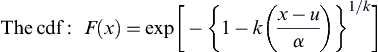(A7.70)

Parameter estimation:

MoM:

For k > 0 (−2 < C_s < 1.14), R² = 1

$k = 0.277648 - 0.322016 C_{s} + 0.060278 C_{s}^{2} + 0.016759 C_{s}^{3} - 0.005873 C_{s}^{4} - 0.00244 C_{s}^{5} - 0.00005 C_{s}^{6}$ $k = 0.277648 - 0.322016 C_{s} + 0.060278 C_{s}^{2} + 0.016759 C_{s}^{3} - 0.005873 C_{s}^{4} - 0.00244 C_{s}^{5} - 0.00005 C_{s}^{6}$

(A7.71)

For k < 0 (−10 < C_s < 0) R² = 0.99998

$k = - 0.50405 - 0.00861 C_{s} + 0.015497 C_{s}^{2} + 0.005613 C_{s}^{3} + 0.00087 C_{s}^{4} + 0.000065 C_{s}^{5}$ $k = - 0.50405 - 0.00861 C_{s} + 0.015497 C_{s}^{2} + 0.005613 C_{s}^{3} + 0.00087 C_{s}^{4} + 0.000065 C_{s}^{5}$

(A7.72)

$\hat{α} = {[m_{2} {\hat{k}}^{2} / {Γ (1 + 2 \hat{k}) - Γ^{2} (1 + \hat{k})}]}^{1 / 2}$ $\hat{α} = {[m_{2} {\hat{k}}^{2} / {Γ (1 + 2 \hat{k}) - Γ^{2} (1 + \hat{k})}]}^{1 / 2}$

(A7.73)

$\hat{u} = m_{1}^{'} - \frac{\hat{α}}{\hat{k}} [1 - Γ (1 + \hat{k})]$ $\hat{u} = m_{1}^{'} - \frac{\hat{α}}{\hat{k}} [1 - Γ (1 + \hat{k})]$

(A7.74)

PWM:

$\hat{k} = 7.8590 C + 2.9554 C^{2}$ $\hat{k} = 7.8590 C + 2.9554 C^{2}$

(A7.75)

where

$C = \frac{2}{3 + t_{3}} - \frac{\ln 2}{\ln 3}$ $C = \frac{2}{3 + t_{3}} - \frac{\ln 2}{\ln 3}$

(A7.76)

$\hat{α} = \frac{l_{2} \hat{k}}{(1 - 2^{- \hat{k}}) Γ (1 + \hat{k})}$ $\hat{α} = \frac{l_{2} \hat{k}}{(1 - 2^{- \hat{k}}) Γ (1 + \hat{k})}$

(A7.77)

$\hat{u} = l_{1} - \frac{\hat{α}}{\hat{k}} [1 - Γ (1 + \hat{k})]$ $\hat{u} = l_{1} - \frac{\hat{α}}{\hat{k}} [1 - Γ (1 + \hat{k})]$

(A7.78)

Quantile estimate: The flood quantile are estimated using the following relationship:

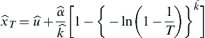${\hat{x}}_{T} = \hat{u} + \frac{\hat{α}}{\hat{k}} [1 - {- \ln (1 - \frac{1}{T})}^{\hat{k}}]$ ${\hat{x}}_{T} = \hat{u} + \frac{\hat{α}}{\hat{k}} [1 - {- \ln (1 - \frac{1}{T})}^{\hat{k}}]$

(A7.79)

A.8. Soil Conservation Services (SCS)–Curve Number (CN) Values (⁶SCS, 1985)

S. No.	Land Use Description/Treatment	Hydrologic Condition/% Impervious Area	Hydrologic Soil Groups
S. No.	Land Use Description/Treatment	Hydrologic Condition/% Impervious Area	A	B	C	D
Urban
1	Residential:
	Average lot size:1/8 acre or less	65	77	85	90	92
	1/4 acre	38	61	75	83	87
	1/3 acre	30	57	72	81	86
	1/2 acre	25	54	70	80	85
	1 acre	20	51	68	79	84
	2 acre	12	46	65	77	82
2	Paved parking lots, roofs, driveways, etc. (excluding right-of-way)		98	98	98	98
3	Streets and roads:
	Paved with curbs and storm sewers (excluding right-of-way)		98	98	98	98
	Paved, open ditches (including right-of-way)		82	89	92	93
	Gravel (including right-of-way)		76	85	89	91
	Dirt (including right-of-way)		72	82	87	89
4	Western desert areas:
	Natural desert landscaping (pervious areas only)		63	77	85	88
	Artificial desert landscaping (impervious weed barrier, desert shrub with 1- to 2-inch sand or gravel mulch and basin borders)		96	96	96	96
5	Urban districts:
	Commercial and business areas	85	89	92	94	95
	Industrial districts	72	81	88	91	93
Table Continued

S. No.	Land Use Description/Treatment	Hydrologic Condition/% Impervious Area	Hydrologic Soil Groups
S. No.	Land Use Description/Treatment	Hydrologic Condition/% Impervious Area	A	B	C	D
6	Developing areas:
	Newly graded areas (pervious areas only, no vegetation)		77	86	91	94
	Idle lands
7	Open spaces, lawns, parks, golf courses, cemeteries, etc.
	Grass cover on 75% or more of the area	Good	39	61	74	80
	Grass cover on 50%–75% of the area	Fair	49	69	79	84
Agricultural
8	Cultivated lands:
	Fallow:
	Bare soil: straight row	–	77	86	91	94
	Crop residue cover	Poor	76	85	90	93
		Good	74	83	88	90
9	Row crops:
	Straight row	Poor	72	81	88	91
	Straight row	Good	67	78	85	89
	Crop residue cover: straight row	Poor	71	80	87	90
	Crop residue cover: straight row	Good	64	75	82	85
	Contoured	Poor	70	79	84	88
	Contoured	Good	65	75	82	86
	Crop residue cover: contoured	Poor	69	78	83	87
	Crop residue cover: contoured	Good	64	74	81	85
	Contoured and terraced	Poor	66	74	80	82
	Contoured and terraced	Good	62	71	78	81
	Crop residue cover contoured and terraced	Poor	65	73	79	81
	Crop residue cover contoured and terraced	Good	61	70	77	80
Table Continued

S. No.	Land Use Description/Treatment	Hydrologic Condition/% Impervious Area	Hydrologic Soil Groups
S. No.	Land Use Description/Treatment	Hydrologic Condition/% Impervious Area	A	B	C	D
10	Small grain:
	Straight row	Poor	65	76	84	88
	Straight row	Good	63	75	83	87
	Crop residue cover straight row	Poor	64	75	83	86
	Crop residue cover straight row	Good	60	72	80	84
	Contoured	Poor	63	74	82	85
	Contoured	Good	61	73	81	84
	Crop residue cover contoured	Poor	62	73	81	84
	Crop residue cover: contoured	Good	60	72	80	83
	Contoured and terraced	Poor	61	72	79	82
	Contoured and terraced	Good	59	70	78	81
	Crop residue cover contoured and terraced	Poor	60	71	78	81
	Crop residue cover contoured and terraced	Good	58	69	77	80
11	Close-seeded legumes or rotation meadow:
	Straight row	Poor	66	77	85	89
	Straight row	Good	58	72	81	85
	Contoured	Poor	64	75	83	85
	Contoured	Good	55	69	78	83
	Contoured and terraced	Poor	63	73	80	83
	Contoured and terraced	Good	51	67	76	80
	Uncultivated lands:
12	Pasture or range:	Poor	68	79	86	89
		Fair	49	69	79	84
		Good	39	61	74	80
	Contoured	Poor	47	67	81	88
	Contoured	Fair	25	59	75	83
	Contoured	Good	6	35	70	79
13	Meadow: continuous grass, protected from grazing, and generally mowed for hay	Good	30	58	71	78
	Brush–brush weed grass mixture with brush being the major element	Poor	48	67	77	83
		Fair	35	56	70	77
		Good	30	48	65	73
14	Farmsteads: buildings, lanes, driveways, and surrounding lots	–	59	74	82	86
Table Continued

S. No.	Land Use Description/Treatment	Hydrologic Condition/% Impervious Area	Hydrologic Soil Groups
S. No.	Land Use Description/Treatment	Hydrologic Condition/% Impervious Area	A	B	C	D
Woods and Forests
15	Humid rangelands or agricultural uncultivated lands:
	Woods or forest land	Poor	45	66	77	83
		Fair	36	60	73	79
		Good	25	55	70	77
16	Woods–grass combination (orchard or tree farm)	Poor	57	73	82	86
		Fair	43	65	76	82
		Good	32	58	72	79
17	Arid and semiarid rangelands:
	Herbaceous	Poor		80	87	93
		Fair		71	81	89
		Good		62	74	85
18	Oak-aspen	Poor		66	74	79
		Fair		48	57	63
		Good		30	41	48
19	Pinyon-juniper	Poor		75	85	89
		Fair		58	73	80
		Good		41	61	71
20	Sagebrush with grass understory	Poor		67	80	85
		Fair		51	63	70
		Good		35	47	55
21	Desert shrub	Poor	63	77	85	88
		Fair	55	72	81	86
		Good	49	68	79	84

Hydrological Soil Group (SCS, 1985)

Group A: The soils falling in Group A exhibit high infiltration rates even when they are thoroughly wetted, high rate of water transmission, and low runoff potential. Such soils include primarily deep, well to excessively drained sands or gravels.

Group B: These soils have moderate infiltration rates when thoroughly wetted and consist primarily of moderately deep to deep, moderately well drained to well-drained soils with fine, moderately fine, to moderately coarse textures, for example, shallow loess and sandy loam. These soils exhibit moderate rates of water transmission.

Group C: Soils in this group have low infiltration rates when thoroughly wetted. These soils primarily contain a layer that impedes downward movement of water. Such soils are of moderately fine to fine texture, for example, clay loams, shallow sandy loam, and soils low in organic content. These soils exhibit a slow rate of water transmission.

Group D: The soils of this group exhibit very low rates of infiltration when they are thoroughly wetted. Such soils are primarily clay soils of high swelling potential, soils with a permanent high water table, soils with a clay pan or clay layer at or near the surface, and shallow soils over nearly impervious material. These soils exhibit a very slow rate of water transmission.

Description of Hydrologic Groups (SCS, 1985)

Hydrologic Soil Group	Minimum Infiltration Rate (cm/h)
A	0.76–1.14
B	0.38–0.76
C	0.13–0.38
D	0–0.13

Description of Hydrologic Conditions (SCS, 1985)

S. No.	Vegetation Condition	Hydrologic Condition
1	Heavily grazed or regularly burned. Litter, small trees, and brush are destroyed.	Poor
2	Grazed but not burned. Some litter exists, but these woods not protected.	Fair
3	Protected from grazing and litter and shrubs cover the soil.	Good

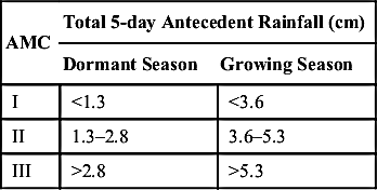
Description of Antecedent Moisture Conditions (SCS, 1985)

AMC	Total 5-day Antecedent Rainfall (cm)
AMC	Dormant Season	Growing Season
I	<1.3	<3.6
II	1.3–2.8	3.6–5.3
III	>2.8	>5.3

Conversion of the CN_II values into CN_I and CN_III.

$C N_{I} = \frac{C N_{I I}}{2.3 - 0.013 C N_{I I}}$ $C N_{I} = \frac{C N_{I I}}{2.3 - 0.013 C N_{I I}}$

(A8.1)

$C N_{I I I} = \frac{C N_{I I}}{0.43 + 0.0057 C N_{I I}}$ $C N_{I I I} = \frac{C N_{I I}}{0.43 + 0.0057 C N_{I I}}$

(A8.2)

where CN_I and CN_III are the CN values corresponding to AMC I and AMC III.

A.9. General Guideline for Embankment Sections (⁷IS 12169, 1987)

S. No.	Description	Height: <5 m		Height: 5–10 m		Height: 10–15 m
1	Type of section	Homogeneous/modified homogeneous section		Zoned/modified homogeneous/homogeneous section		Zoned/modified homogeneous/homogeneous section
2	Side slopes	U/S	D/S	U/S	D/S	U/S	D/S
(a)	Coarse grained soil
	(i) GW, GP, SW, SP	Not suitable		Not suitable		Not suitable for core, suitable for casing zone
	(ii) GC, GM, SC, SM	2:1	2:1	2:1	2:1	Section to be decided based on stability analysis
(b)	Fine grained soil
	(i) CL, ML, CI, MI	2:1	2:1	2.5:1	2.25:1	Section to be decided based on stability analysis
	(ii) CH, MH	2:1	2:1	3.75:1	2.5:1	Section to be decided based upon stability analysis
3.	Hearting zone	Not required		May be provided		Necessary
	(a) Top width	–		3 m		3 m
	(b) Top level	–		0.5 m above MWL		0.5 m above MWL
4.	Rock toe height	Not necessary up to 3 m height. Above 3 m height, 1 m height of rock toe may be provided		Necessary = H/5		Necessary = H/5
5.	Berms	Not necessary		Not necessary		The berm may be provided as per design. The minimum berm width shall be 3 m.

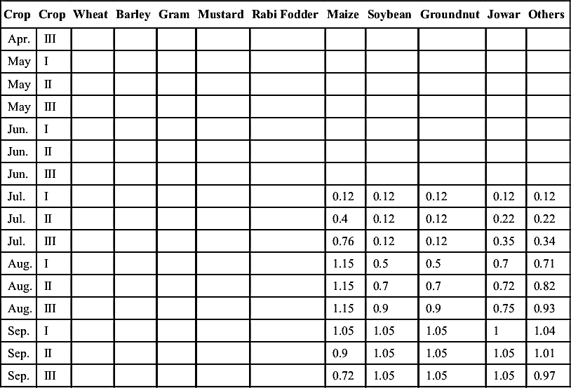
A.10. 10-Daily Crop Coefficients For Major Crops Of Rabi And Kharif Seasons (Dimensionless)

Crop	Crop	Wheat	Barley	Gram	Mustard	Rabi Fodder	Maize	Soybean	Groundnut	Jowar	Others
Month	Duration of crop	130	130	141	130	182	102	130	130	115	140
10-Day/date of sowing		16-Nov.	07-Nov.	21-Oct.	16-Oct.	16-Oct.	01-Jul.	01-Jul.	01-Jul.	01-Jul.	01-Jul.
Oct.	I						0.6	1.05	1.05	0.75	0.75
Oct.	II				0.1	0.5	0.5	0.9	0.9	0.6	0.6
Oct.	III			0.1	0.1	0.66		0.75	0.75	0.5	0.5
Nov.	I		0.2	0.3	0.2	0.65		0.2	0.2
Nov.	II	0.2	0.2	0.8	0.54	0.65
Nov.	III	0.3	0.75	0.8	0.54	0.85
Dec.	I	0.75	0.75	1.05	0.9	0.9
Dec.	II	0.84	0.75	1.1	0.95	0.8
Dec.	III	1.05	0.75	1.1	1	0.6
Jan.	I	1.15	1.05	1.1	1.1	0.8
Jan.	II	1.15	1.15	1.05	1.15	0.65
Jan.	III	1.15	0.65	0.8	0.9	0.54
Feb.	I	1.15	0.65	0.55	0.8	0.8
Feb.	II	1.15	0.65	0.55	0.6	0.65
Feb.	III	0.9	0.25	0.25	0.4	0.6
Mar.	I	0.84	0.2			0.85
Mar.	II	0.4	0.2			0.75
Mar.	III	0.2				0.6
Apr.	I					0.85
Apr.	II					0.75
Table Continued

Crop	Crop	Wheat	Barley	Gram	Mustard	Rabi Fodder	Maize	Soybean	Groundnut	Jowar	Others
Apr.	III
May	I
May	II
May	III
Jun.	I
Jun.	II
Jun.	III
Jul.	I						0.12	0.12	0.12	0.12	0.12
Jul.	II						0.4	0.12	0.12	0.22	0.22
Jul.	III						0.76	0.12	0.12	0.35	0.34
Aug.	I						1.15	0.5	0.5	0.7	0.71
Aug.	II						1.15	0.7	0.7	0.72	0.82
Aug.	III						1.15	0.9	0.9	0.75	0.93
Sep.	I						1.05	1.05	1.05	1	1.04
Sep.	II						0.9	1.05	1.05	1.05	1.01
Sep.	III						0.72	1.05	1.05	1.05	0.97

A.11. Field Capacity and Permanent Wilting Point

S. No.	Texture	Field Capacity, FC (%)	Permanent Wilting Point, PWP (%)
1	Sand	10	5
2	Loamy sand	12	5
3	Sandy loam	18	8
4	Sandy clay loam	27	17
5	Loam	28	14
6	Sandy clay	36	25
7	Silty loam	31	11
8	Silt	30	6
9	Clay loam	36	22
10	Silty clay loam	38	22
11	Silty clay	41	27
12	Clay	42	30

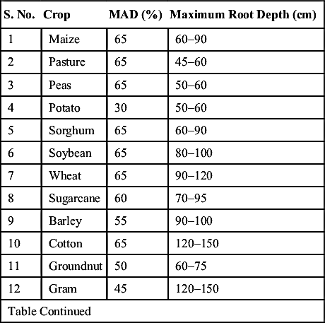
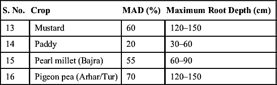
A.12. Values of Maximum Allowable Deficit and Root Depth of Crops

S. No.	Crop	MAD (%)	Maximum Root Depth (cm)
1	Maize	65	60–90
2	Pasture	65	45–60
3	Peas	65	50–60
4	Potato	30	50–60
5	Sorghum	65	60–90
6	Soybean	65	80–100
7	Wheat	65	90–120
8	Sugarcane	60	70–95
9	Barley	55	90–100
10	Cotton	65	120–150
11	Groundnut	50	60–75
12	Gram	45	120–150
Table Continued

S. No.	Crop	MAD (%)	Maximum Root Depth (cm)
13	Mustard	60	120–150
14	Paddy	20	30–60
15	Pearl millet (Bajra)	55	60–90
16	Pigeon pea (Arhar/Tur)	70	120–150

A.13. Approximate Net Irrigation Depth Applied per Irrigation (mm)

Soil Type	Shallow Rooted	Medium Rooted	Deep Rooted
Shallow and/or sandy soil	15	30	40
Loamy soil	20	40	60
Clayey soil	30	50	70

A.14. Recommended Value of Irrigation Application Rate

Soil Type	Maximum Application Rate With Different Land Slopes (mm/h)
Soil Type	0%–5%	5%–8%	8%–12%
Coarse sandy soil	38.0–50.8	25.4–38.1	19.0–25.4
Light sandy	19.0–25.4	12.7–20.3	10.2–15.2
Silt loam	7.62–12.7	6.35–10.2	3.81–7.62
Clay loam to clay	3.81	2.54	2.03

..................Content has been hidden....................

You can't read the all page of ebook, please click here login for view all page.

Table of Contents for Appendices

Create new playlist

Sign In

Sign Up

Appendices

A.1. Unit Conversion Factor

A.2. (A) Guidelines for Interpretations of Water Quality Parameters for Irrigation (1FAO, 1994)

(B) Usual Range of Water Quality Parameters for Irrigation (2FAO, 1994)

A.3. FORTRAN Program for Mann–Kendal Test

A.4. Guidelines for Selecting the Design Floods (3CBIP, 1989)

A.5. Computation of Design Flood for Medium to Small Irrigation Project: Unit Hydrograph Technique

A.6. Computation of Design Flood for Microirrigation Projects: SCS-CN Method

A.7. Computation of Design Flood: Statistical Distribution Used in Frequency Analysis

1. Normal Distribution

2. Log-Normal Distribution

3. Two-Parameter Gamma Distribution

4. Pearson (3) Distribution

5. Log-Pearson (3) Distribution

6. Extreme Value Type I Distribution (Gumbel Distribution)

7. Generalized Extreme Value Distribution

A.8. Soil Conservation Services (SCS)–Curve Number (CN) Values (6SCS, 1985)

Hydrological Soil Group (SCS, 1985)

Description of Hydrologic Groups (SCS, 1985)

Description of Hydrologic Conditions (SCS, 1985)

Description of Antecedent Moisture Conditions (SCS, 1985)

A.9. General Guideline for Embankment Sections (7IS 12169, 1987)

A.10. 10-Daily Crop Coefficients For Major Crops Of Rabi And Kharif Seasons (Dimensionless)

A.11. Field Capacity and Permanent Wilting Point

A.12. Values of Maximum Allowable Deficit and Root Depth of Crops

A.13. Approximate Net Irrigation Depth Applied per Irrigation (mm)

A.14. Recommended Value of Irrigation Application Rate

Table of Contents for
Appendices

A.2. (A) Guidelines for Interpretations of Water Quality Parameters for Irrigation (¹FAO, 1994)

(B) Usual Range of Water Quality Parameters for Irrigation (²FAO, 1994)

A.4. Guidelines for Selecting the Design Floods (³CBIP, 1989)

A.8. Soil Conservation Services (SCS)–Curve Number (CN) Values (⁶SCS, 1985)

A.9. General Guideline for Embankment Sections (⁷IS 12169, 1987)