Chapter 5

One-dimensional Problems

Life is complex – it has both real and imaginary parts.

Anonymous

5.1  INTRODUCTION

We have seen in earlier chapters that microscopic particles always manifest themselves in the form of waves: depending upon the situation the wave could be an extended plane wave or could be in the form of a wave packet. The form of these waves may be obtained by solving the corresponding Schrodinger equation of the particle under the given conditions. In this chapter, we shall study dynamics of a particle in one-dimensional space under a given potential field, that is, we shall find out energy eigenvalues and eigenfunctions of the Hamiltonian operator. But firstly we shall discuss some of the general features of the eigenfunctions.

5.2  TIME-INDEPENDENT SCHRODINGER EQUATION AND STATIONARY STATES

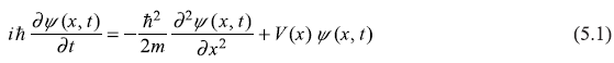
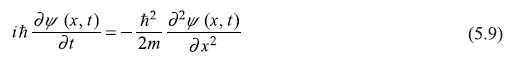
Let us consider one-dimensional version of time-dependent Schrodinger equation obtained in Chapter 4:

Let us consider the special case of a closed system in which energy is conserved and the potential energy V is time-independent, that is, the Hamiltonian of the system is independent of time. In such case, we shall see, it would be possible to solve Eq. (5.1) by reducing it to a pair of ordinary differential equations in one variable. Let us use the method of separation of variables in writing

 

 

Putting Eq. (5.2) in Eq. (5.1), we get

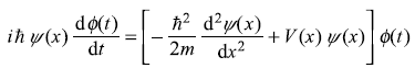
Dividing by ψ(x) ϕ(t) on both sides gives

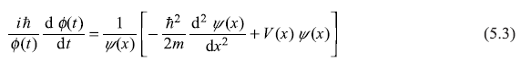
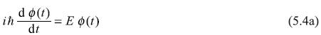
The L.H.S. of this equation is a function of time alone, whereas the R.H.S. is a function of space alone and so both sides must be equal to a constant, which we call E. Thus we get two equations:

and

Equation (5.4a) is the time-dependent Schrodinger equation and Eq. (5.4b) is time-independent Schrodinger equation. The solution to the time-dependent equation is of simple harmonic form

 

 

From Eq. (5.2), we have

 

 

We notice a very important point here. The Schrodinger equation dictates that (for a closed system when the potential energy V is time independent) the time dependence of the wave function is through the exponential factor e^–iωt. Any alternatives such as e^iωt or trigonometric functions such as sin (ωt) or cos (ωt) are simply not admissible. For example, in case of a free particle propagating in x-direction, where time-independent wave function is

 

 

the time-dependent wave function shall be

 

 

Any of the following form of time-dependent wave function is not admissible.

 

 

 

 

It can be easily verified that none of the above three forms is a solution of time-dependent Schrodinger equation for free particle

Returning back to the time-dependent wave function [Eq. (5.6)], it may be noted that the probability density |ψ(x, t)|² is really independent of time. So the wave function ψ(x, t) = [ψ(x) ϕ(t)] is called a stationary state.

The time-independent Schrodinger Eq. (5.4b) may be written as eigenvalue equation

where

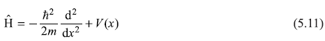
is the Hamiltonian operator and E is a number, giving energy eigenvalue. In general, the eigenvalues have a discrete set with corresponding eigenfunctions and, therefore, Eq. (5.10) may be written as

So, for a particle in a given potential V(x), the solution of Schrodinger equation shall give a number of stationary states (i.e., the eigenstates) in which the particle may stay.

5.3  SOME CHARACTERISTICS OF WAVE FUNCTIONS

5.3.1  Finiteness of Wave Functions

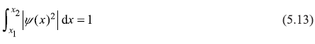
It was argued in Section 4.3 that the wave function ψ(x), interpreted as probability amplitude is, in general, complex and therefore can not be matched with any observable physical quantity. However, |ψ(x)|² is real and |ψ(x)|² dx gives information about the probability of particle being found in between positions x and x + dx. |ψ(x)|² gives probability density of the particle at position x and, therefore, ψ(x) should be single valued. If a particle is confined within a region from x₁ to x₂ with its wave function ψ(x) in this region, then (as total probability of the particle being found anywhere within the region of x₁ to x₂ has to be unity)

Also |ψ(x)|² dx has to have a finite value for finite value of dx. Therefore, the condition

 

 

dictates that ψ(x) has to have finite value everywhere in the region, that is, the wave function ψ(x) shall not diverge at any value of x.

5.3.2  Continuity of Wave Functions

Not only the wave function ψ(x) should be finite everywhere in the region, ψ(x) as well as its derivative (dψ/dx) should be continuous. The discontinuity in the wave function ψ(x), for example, shown in Figure 5.1, would result in a non-physical situation. In fact, the infinite slope of the wave function at x = x_o would result in the infinite contribution to the expectation value of the particle’s kinetic energy.

5.3.3  Orthogonality of Wave Functions

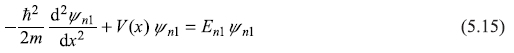
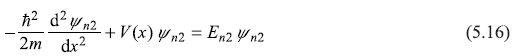
We shall see here that all eigenfunctions of a Hermitian operator (Hamiltonian is a Hermitian operator) corresponding to different eigenvalues (which are real) are orthogonal. Let us consider a particle in a one-dimensional potential V(x). The Schrodinger equations corresponding to the two eigenvalues E_n1 and E_n2 with corresponding eigenstates ψ_n1(x) and ψ_n2(x) are:

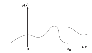
Figure 5.1 An unacceptable form of wave function ψ(x) as at x = x_o, (dψ/dx) = ∞

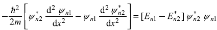
Let us multiply Eq. (5.15) by and multiply the complex conjugate of Eq. (5.16) by ψ_n1, and take the difference of the two resulting equations. We get

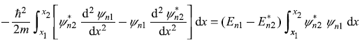
Integrating between the limits x₁ and x₂, we get

or

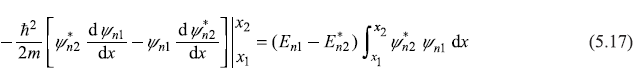
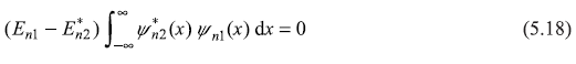
If we take x₁ = –∞ and x₂ = ∞, the L.H.S. of (5.17) vanishes, as ψ_n1 and ψ_n2 are eigenfunctions and they are zero at ± ∞. So

If n₁= n₂, the integral dx is definte positive (in fact if ψ_n1 is a normalized wave function), so

clearly showing that E_n1 is real and hence all energy eigenvalues are real. Eq. (5.18) for E_n1 ≠ E_n2 gives

Two functions, ψ_n1(x) and ψ_n2(x) having this property [Eq. (5.20)] are called orthogonal to each other. If each ψ(x) is normalized, we may write

where δ_{n1, n2} is called the Kronecker delta function defined through the equation

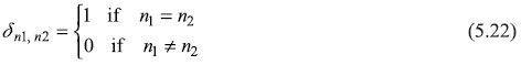
Two functions which satisfy Eq. (5.21) are orthogonal and normalized, and simply called orthonormal.

5.4  PARTICLE IN A ONE-DIMENSIONAL POTENTIAL BOX

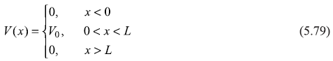
Let us firstly consider a very simple case of a particle in a one-dimensional potential box. We shall solve the Schrodinger equation of a particle of mass m confined in a potential box of length L. The potential is expressed as

 

 

The situation is analogous to a classical system of a ball put inside a gravitational well of infinite depth. The ball is moving on the (frictionless horizontal) floor along x-axis only. There are vertical impenetrable rigid walls at x = 0 and x = L. The motion of this classical ball is oscillatory along x-axis, being repeatedly reflected by walls at x = 0 and x = L. Of course, in this example of classical ball in a gravitational wall, both the size of the ball and the length of the well L are macroscopic quantities of the order of centimetres and meters, respectively.

In case of microscopic particle (say electron, proton, or atomic ion) in a potential well, the length L of potential well is very small of the order of a few nanometres. The particle might be moving along x-axis in the form of some wave packet. We have to find the form as well as the energy of the wave packet, obviously by solving Schrodinger equation of the particle. By now, we are sure any information about the particle may only be obtained from its Schrodinger equation.

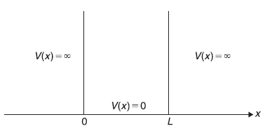
Figure 5.2 A one dimensional potential box, that is, a potential well with infinitely high potential barriers on both sides

5.4.1  Energy Eigenvalues and Eigenfunctions

The one-dimensional time-independent Schrodinger equation of the particle inside the well, where V = 0, is

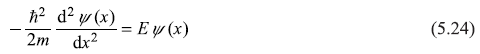
As the potential energy V(x) is infinite outside the well, that is, for x < 0 and for x > L, the probability of finding the particle outside the well is zero. Therefore, the wave function ψ(x) should vanish outside the well. And, in fact, we need to solve Schrodinger Eq. (5.24) only inside the well. We have learnt earlier in Section 5.3 that the wave function must be continuous and, therefore, ψ(x) must vanish at the well boundaries, that is,

 

 

The conditions (5.25) are known as rigid boundary conditions. Particle in a box may also be considered under, what are known as periodic boundary conditions. We shall consider a particle in a potential box within periodic boundary conditions in the next section. In fact, we shall learn shortly that it is the boundary conditions (5.25) which lead to the discrete values of energy of the particle. And later on, we shall see that in all cases it is the boundary condition(s) only which dictate the energy of the particle to have discrete values.

Eq. (5.24) may be written as

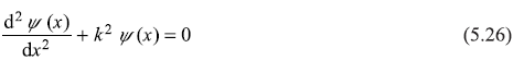
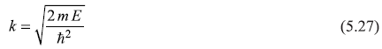
where

The general solution of second order differential equation [Eq. (5.26)] is a linear combination of two linearly independent solutions exp(ikx) and exp(–ikx). So

 

 

where A and B are arbitrary constants. These constants are to be fixed by the boundary conditions (5.25), which give

 

 

and

 

 

From these two equations, we get

 

 

or

 

 

which dictates that only allowed values of k are k_n, given by

 

 

So the wave function [Eq. (5.28)], with condition [Eq. (5.29a)] (B = –A) and with allowed values of k given by Eq. (5.30b), becomes

 

 

Now normalization of ψ_n(x) means

or

or

or

Therefore, we get the normalized wave function

It may be noted here that the following expressions of ψ_n (x) are equally valid

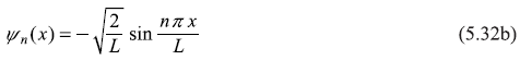
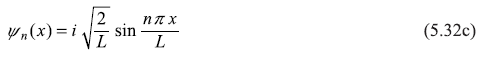
This is so because the position probability density |ψ(x)|² obtained from any of the above expressions is same and it is only probability density (and not the wave function) which is to be compared with the experimental results. In fact, the wave function could be real, imaginary, complex, positive, or negative; it does not matter.

5.4.1.1  An alternative way of solving Eq. (5.26)

It may be more convenient in this case to solve Schrodinger equation to start with real general solutions, that is,

 

 

where arbitrary constants A and B are to be found using two boundary conditions

 

 

These two equations give (as in the earlier method)

 

 

with allowed of k given by

 

 

So the wave function (5.33) becomes

 

 

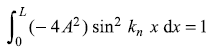
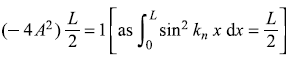
Normalization of ψ_n(x) shall give

so

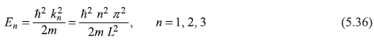
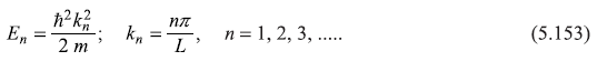
The energy of the particle E [= (ħ²k²)/2m, Eq. (5.27)] has discrete values as wave vector k has discrete values k_n [= (n π) / L].

We see the eigen energy spectrum of the particle consists of infinite number of discrete energy levels E₁, E₂, ... corresponding to bound eigenstates ψ₁, ψ₂, ... That ψ₁, ψ₂, ψ₃..., are called bound states, is clear because the particle in these states is confined within the box. Later on we shall explain unbound states when we shall consider particle in a potential well of finite depth.

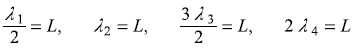
Let us see how the real wave function ψ_n(x) looks like for different values of n. In Figure 5.3, we plot ψ₁, ψ₂, ψ₃ ... and show corresponding energies E₁, E₂, E₃......We know that the wave vector k_n is quantized k_n = (nπ)/L. The corresponding de Broglie wavelengths are λ_n = (2π)/k_n = (2L)/n. So only those states are allowed in which either half an odd intergal or integral number of de Broglie wavelengths fit into the box of length L. Like

Also, we note that as energy increases, number of nodes in that state increases. Precisely, the eigenstate ψ_n(x) with energy eigenvalue E_n has (n – 1) nodes within the potential well (leaving the nodes at the boundaries).

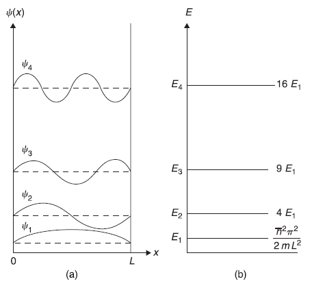
Figure 5.3 (a) First four eigenfunctions of the particle in the infinite potential well. (b) corresponding four eigenvalues

5.4.2  Orthogonality of Wave Functions

We may easily check that different wave functions are orthogonal to each other.

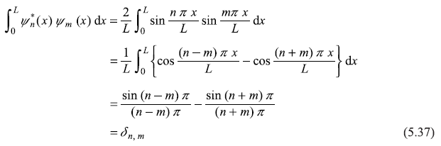
where δ_{n, m} is the Kronecker delta-function.

 

and

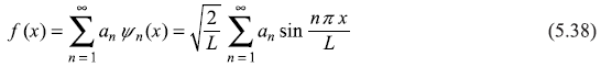
5.4.3  Completeness Condition

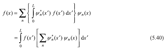
The eigenfunctions ψ_n(x) form a discrete set. The infinite number of discrete eigenfunctions given by Eq. (5.32) form a complete set in the sense that an arbitrary function f(x) [satisfying the boundary conditions as the eigenfunctions do, viz f(0) = f(L) = 0] can be expanded in terms of ψ_n(x):

The coefficients a_n may be found by multiplying above equation by and integrating from 0 to L:

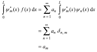
Thus

Substituting expression of a_n from Eq. (5.39) in Eq. (5.38), we get

Now using one of the properties of Dirac delta-function δ(x – x′), we have

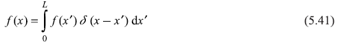
Comparing Eqs (5.40) and (5.41), we may write

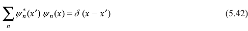
representing the completeness condition of eigenfunctions ψ_n(x)of Eq. (5.32).

5.4.4  Position Probability Density

For nth state, the position probability density P_n(x) is given as

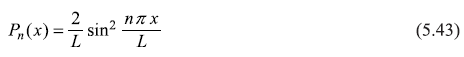
In Figure 5.4, we show schematic plot of position probability density P₁(x), P₂(x), P₃(x), and P₄(x). Let us discuss explicitly the meaning of probability density. As per the usual definition of probability, if an identical experiment is repeated N times (e.g., a single coin is tossed repeatedly N-times), then we define probability of a particular event as equal to the number of favourable events divided by N (the total number of events). With this definition in mind, we shall prepare N identical potential wells each of width L, with one (identical) particle in each. Let us have particle in same state ψ_n(x) in each well. In each well, the length L is divided (say) in 20 equal intervals. Particle in each box is observed by separate observers. Each observer will report about the particular interval, he observed particle in. When these N observations are plotted, we will find exactly similar curve as that of P_n(x). For example, if the particle is put in ψ₂(x) state, no observer will find particle at position x = L/2.

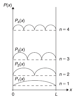
Figure 5.4 Schematic plot of first four position probability densities

5.4.5  Expectation Values of Linear Momentum and Kinetic Energy Operators

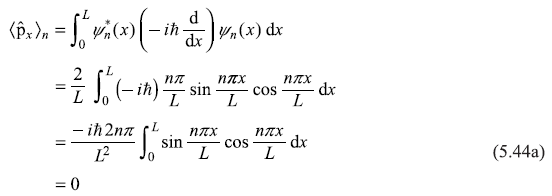
We had learnt in Chapter 4 that in quantum mechanics a physical quantity is obtained by finding the expectation value of the corresponding operator. We also know the operator corresponding to the physical quantity p_x, the x-component of linear momentum. So, let us find the expectation value of the operator in state ψ_n.

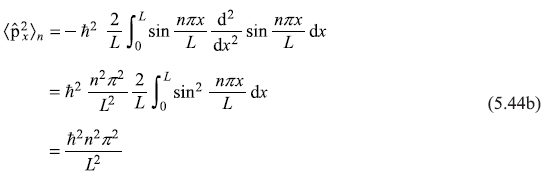
However, the expectation value of is

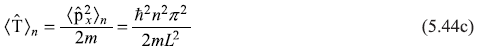
And expectation value of kinetic energy operator is

In the beginning, it may seem to be surprising to see that value of is zero, whereas that of is non-zero. But, one may understand it as the eigenstate is really representing (not a running wave but) a standing wave.

In fact, we should write time-dependent eigenstate to see what type of wave the eigenstate represent.

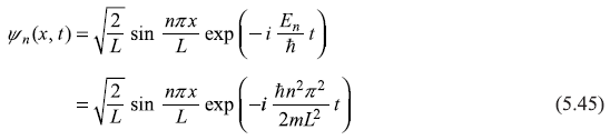
Now, it can be easily checked that ψ_n(x, t) is representing a standing wave and not a running wave. For example, at x₁ = L/n, the wave function ψ_n(x) is zero at all times, a node there; characteristic of standing wave in classical physics. So just like in classical mechanics, expression (5.45) may be thought of superposition of two propagating waves of equal wavelength and frequency: (i) one propagating in +x direction and (ii) the other (after reflection at x = L) propagating in –x direction. Each of the two constituent waves (i) and (ii) carry equal and opposite linear momentum and, therefore, net linear momentum carried is zero. So

5.4.6  Uncertainty Relation Built in Schrodinger Equation

The minimum energy obtained for a particle in potential box is

It may be noted that while writing for the allowed values of k, we wrote in Eq. (5.30b)

 

 

and n = 0 was not included in Eq. (5.30b). It may be easily checked that for n = 0 the eigenstate

and ψ₀(x) = 0 means the particle has probability zero to be found in state n = 0, so n = 0 is not allowed, simply.

Now, if we apply Heisenberg’s uncertainty principle to a particle in the potential box, we notice

 

 

(as particle could be anywhere in length L)

 

∴

and the minimum kinetic energy of the particle is

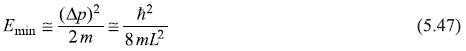
But, as potential energy of the particle in the box is zero, E_min is the (minimum) total energy, which is estimated to be of same order of magnitude as E₁ obtained from the Schrodinger equation. Obviously, Schrodinger equation contains the spirit of the uncertainty principle in it.

5.5  POTENTIAL BOX WITH PERIODIC BOUNDARY CONDITIONS

In the previous section, we discussed states of a particle in a one-dimensional potential box [defined through Eq. (5.23)] with rigid boundary conditions [specified by Eq. (5.25)]. Under these conditions, the particle is confined (or bound) within the box. If we consider some practical cases like conduction electrons in simple metals, the electrons are almost free to move when well within the metal. But, when the electron reaches the boundary of the metal, that is, near the metal surface, it experiences a rise in potential. We may assume the conduction electrons to be free in the metal, in reality there is a weakly varying periodic potential which the conduction electrons feel. However, the simple free electron model works. So, conduction electrons are in a sort of potential well of finite depth. Now, when we discuss any electronic property of a metal (e.g., electrical conductivity, electronic specific heat, etc.), we hardly mention shape or size of the metal. Therefore, we would like to have description of electrons in a metal, which does not include surface or boundary effects. This may be achieved by considering electrons inside metal as electrons inside a potential well with periodic boundary conditions.

In periodic boundary conditions, we assume that as and when a propagating electron in state ψ(r) leaves one end of the metal (or one end of the potential well), another electron enters the other end of the metal (or other end of the well) in the same state. So, in a way we assume here that there is no effect of the boundaries of the potential well on propagation of electrons. Here we shall consider only one-dimensional case which shall correspond to a one-dimensional metal. So, let us consider a particle in a one-dimensional potential well (or box) of width L. Then the periodic boundary conditions, mathematically, mean that the wave function of the particle follows following condition:

 

5.5.1  Energy Eigenvalues and Eigenfunctions

Firstly let us find out energy eigenvalues and eigenfunctions of the particle by solving the Schrodinger equation

along with the boundary conditions given by Eq. (5.48). The general solution of Eq. (5.24) may be written as

 

 

where k is given by Eq. (5.27). Now, we notice that within periodic boundary conditions, the propagating particle (wave) is not affected by the boundary (at x = 0 and x = L), that is, it is not reflected back. Therefore, only one of the two terms of Eq. (5.28) is there. So

 

 

Applying periodic boundary conditions (5.48) on this wave function, we get

 

 

or

 

 

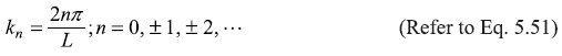
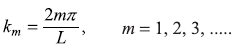
So allowed values of k are k_n, given by

 

 

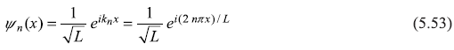
The wave function (5.49) becomes

 

 

It is easy to find out the normalization constant A.

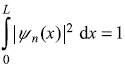
or

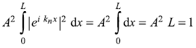
or

Therefore, the normalized wave function is

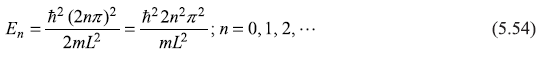
The energy eigenvalues have values

5.5.2  Orthogonality of Wave Functions

Let us find out the integral

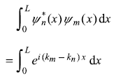
So wave functions are orthonormal.

5.5.3  Position Probability Density

The position probability density P_n(x) for the n-th state may be written as [using Eq. (5.53)]

The position probability density of the particle in the potential well with periodic boundary conditions is totally different than that found with rigid boundary conditions. As Eq. (5.56) dictates, the P_n(x) here is totally x-independent. That means the particle density is uniformly spread within the well. That further means the particle is equally probable to be found anywhere within the well (when one performs some experiment to detect the particle position inside the well).

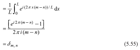
5.5.4  Expectation Values of Linear Momentum and Kinetic Energy Operators

The expectation value of (x-component) of linear momentum operator in n-th state is:

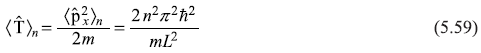
The expectation value of is

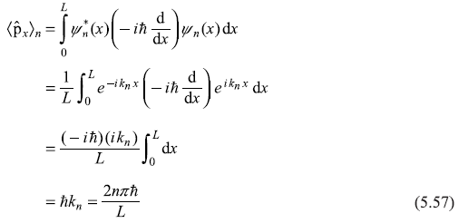
And expectation value of kinetic energy operator is

5.5.5  Uncertainty Relations

Let us discuss marked difference between the results of applying two different boundary conditions, viz. the rigid boundary conditions (RBC) and the periodic boundary conditions (PBC). For example, in the former case, the allowed values of wave vector k_n are

whereas for the latter case, the allowed values are

Notice that n = 0 is not allowed in the former case, whereas n = 0 is allowed in the latter case. For n = 0, the wave function for rigid boundary conditions vanishes

while for periodic boundary conditions, we have

For the RBC case, the solution of Schrodinger equation dictates that it is not possible to have minimum energy of the particle E_o to be zero as it would have violated the uncertainty principle. With the rigid boundary conditions, the particle is confined within the width of the well, that is, ∆x = L and, therefore, the Schrodinger equation has rightly given the solution such that minimum energy of the particle is (in agreement with uncertainty principle).

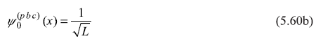
For the PBC case, the solution of Schrodinger equation suggests, it is possible to have value of n to be zero and, therefore, minimum energy of the particle E_o may be zero. This is again in agreement with the uncertainty principle. In fact, with PBC, the particle is not confined within the well. The particle (wave) crosses the boundary and goes on propagating. But a second particle (wave) enters the other boundary so that one particle always remains in the well: giving rise to the normalization constant a value of Therefore, the particle (wave) is propagating in the same direction (without being affected by the boundary) and it is an infinitely extended wave. In fact, particle is free to move in infinite space. So ∆x = ∞, giving E_min = 0.

Therefore, it becomes clear that the wave function is a free particle wave function (of course, normalized within length L).

5.6  THE POTENTIAL STEP

Let us consider one-dimensional motion of a particle in a potential V(x) which has constant value V_o in a (infinitely wide) region x > 0. For x < 0, V(x) = 0. (See Figure 5.5).

Before discussing quantum mechanical case, let us discuss briefly the motion of a classical particle (say a small block of mass m) moving in x-direction with initial kinetic energy E on a frictionless floor as in Figure 5.6 which shows a (gradual) step (gravitational) potential V(x). If the initial energy of the particle (coming from left) is E = E₁ < V₀, the block shall come up to a point (say x₁) where E₁= V(x₁) and then shall be reflected back. The region to the right of x₁ is, in fact, forbidden by the laws of classical mechanics. Total energy E of the particle can not be lesser than its potential energy at a point. The position x₁ may be called as classical turning point and here the kinetic energy of the particle vanishes. However, if E = E₂ >V_o, the block goes on moving in +x direction, of course, with lesser kinetic energy (E₂ – V_o).

We now return to the case of quantum mechanical study of the motion of a microscopic particle of kinetic energy E incident from left on the step up potential (Figure 5.5). The potential for quantum mechanical case is taken to be, step up and not the smoothly increasing (gravitational) potential of classical mechanical example only because it is simple to solve Schrodinger equation for potential given by Figure 5.5,

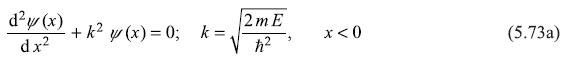
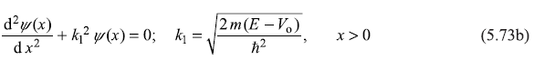
The one-dimensional time-independent Schrodinger equation of the particle is

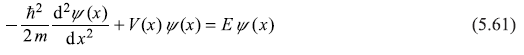
where

 

 

By solving Schrodinger equation for the given potential, we wish to obtain ψ(x) for all x. Let us divide the x-axis into two domains: region I (x < 0) and region II (x > 0) as shown in Figure 5.5. The Schrodinger equation shall be solved for two cases, E < V_o and E > V_o.

5.6.1  Case I: E < V _o

For the two regions I and II, the Schrodinger equation becomes

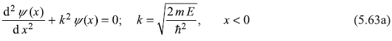
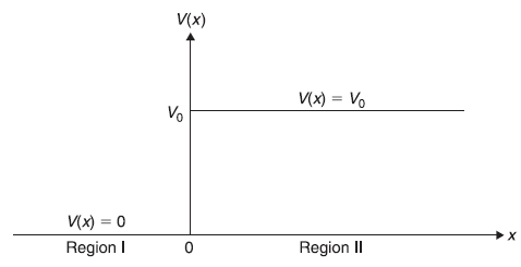
Figure 5.5 A one-dimensional step potential

Figure 5.6 A one-dimensional (gradual) step potential

and

Equation (5.63a) in region I (x < 0), describing the motion of a free particle of wave number k, has general solution

 

 

Equation (5.63b) in region II has general solution

 

 

Here A, B, C, and D are arbitrary constants. Looking at Eq. (5.64b), we conclude that if C ≠ 0, the eigenfunction ψ_II(x) for x > 0 shall diverge in the limit x → +∞, therefore, C = 0.

And we have

 

 

As discussed in Section 5.3, eigenfunction ψ(x) and its first derivative dψ/dx should be finite and continuous for all values of x. Therefore, at x = 0 the solutions (5.65a) and (5.65b) should join smoothly such that ψ(x) and are continuous across x = 0. For the eigenfunction to be continuous at x = 0, we have ψ_I(0) = ψ_II(0) giving the relation

 

 

whereas for the derivative of eigenfunction to be continuous at x = 0, we have dψ_I/dx|_{x = o} = dψ_II/dx |_{x = o}

which gives

 

 

From Eqs (5.66), we get

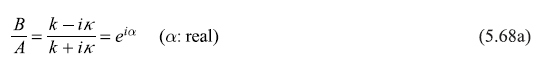
It may be easily seen that

Substituting these values in Eq. (5.65), we get

Figure 5.7 shows schematic plot of wave function ψ(x) given by Eqs (5.69).

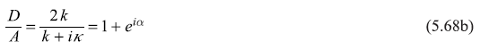
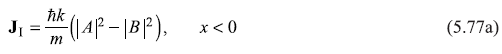
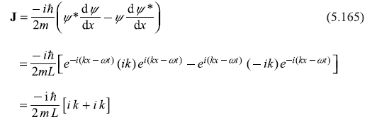
The wave function obtained [Eq. (5.65)] can be easily given a physical interpretation. It represents a plane wave of amplitude A propagating towards right and a reflected wave of amplitude B propagating towards left. In fact, the function e^ikx when multiplied by the factor e^–iEt/ħ represents a plane wave moving in +x direction. Now, we consider the probability current density J associated with the wave function (5.65a). We know that probability current density is given by

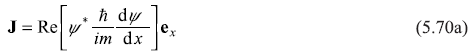
For wave function (5.65a) J comes out to be

 

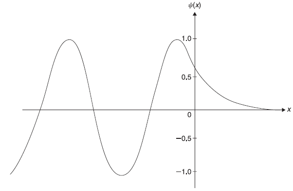
Figure 5.7 Plot of wave function ψ(x) given by Eqs (5.69) with A = 1/2 exp(–ia/2)

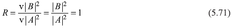
where v = ħ k/m is the magnitude of velocity of the particle. The reflection coefficient R is defined as the ratio of the reflected probability current density v|B|² to the incident probability current density v|A|². So and the reflection is total. It may be noted that the corresponding result of classical mechanics is also same. According to classical mechanics, all particles, each with total energy E < V_o, incident on the potential step, shall be reflected back completely.

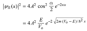
The position probability density in region I and II may be written as

 

P_I(x) shows oscillatory behaviour, which results from interference effect between the (quantum mechanical) incident and reflected waves. P_II(x) decreases exponentially with increasing x in region II. So, we have finite probability of particle being found in classical forbidden region x > 0. We shall see in next sections the importance of this non-classical phenomenon of barrier penetration.

5.6.2  Case 2: E > V_o

Let us now turn to the case when energy of the incident particle E is greater than V_o. The Schrodinger equation for regions I and II becomes

and

These equations have general solution

 

 

 

The term Ae^–ikx and Ce^–ik₁x represent the waves propagating in the +x direction while the terms, Be^–ikx and De^–ik₁x represent the waves propagating in –x direction. This may be easily seen by multiplying these terms by the time dependent factor e^–Et/ħ. Here we are considering the particle (wave) incident from the left of the barrier at x = 0. There can not be a reflected wave in the region II (x > 0) so we must set D = 0. Now the eigenfunction ψ(x) and its first derivative (dψ/dx) must be continuous at x = 0. This gives

 

and

 

From Eqs (5.75), we get

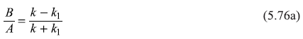
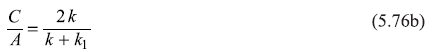
Now, the probability current density J (Eq. 5.70a) for wave functions of Eqs (5.74a) and (5.74b) come out to be

Here

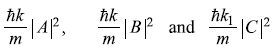
represent the magnitude of probability current densities associated, respectively, with the incident wave (Ae^ikx), reflected wave (Be^–ikx) and the transmitted wave(Ce^ik₁x). The reflection and transmission coefficients, R and T are given by

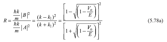
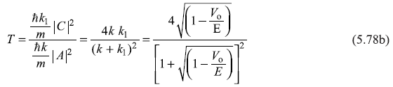
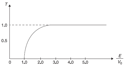
Figure 5.8 Schematic plot of transmission coefficient T as a function of E/V_o for a step potential

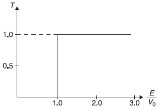
Figure 5.9 Transmission coefficient T as a function of E/V_o for classical case

We may note that R + T = 1 (as it should be).

We now plot in Figure 5.8 the transmission coefficient T as a function of E/V₀, including the case of E/V₀ < 1, for which R = 1, as shown in Eq. (5.71).

In Figure 5.9, we show, for comparison, the transmission coefficient T of a particle incident on a step potential but following classical mechanics. Here for E < V₀, the particle will not be transmitted (i.e., T = 0; same as in quantum mechanical case); but for E > V₀, the particle will be transmitted with probability 1 (i.e., T = 1; different than that in quantum mechanical case).

5.7  RECTANGULAR POTENTIAL BARRIER

We now consider a potential barrier of finite width as shown in Figure 5.10.

The potential is described as

The classical mechanics tells us that a particle incident on this barrier (from left) with its (total) energy E, would be reflected back if E < V₀ and would be transmitted if E > V₀. We expect totally different results for a microscopic particle incident on the barrier (in both cases E < V₀ as well as E > V₀) for which quantum mechanics is to be applied. In fact, we shall see, the application of quantum mechanics to the problem leads to the conclusion that the reflection and transmission take place (with finite probability) for both cases viz. E < V₀ and E > V₀.

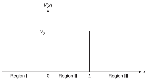
Figure 5.10 A rectangular potential barrier of height V₀ and width L

5.7.1  Case I: E < V₀

For E < V₀, the general solutions of Schrodinger equation in the three regions may be written as

 

 

 

 

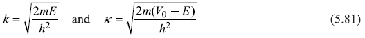
where again

As in the previous section, we assume the particle be incident from left, so there can not be a reflected wave (propagating in –x direction) in region III, and we must set G = 0. The eigenfunction ψ and its derivation dψ/dx must be continuous at points x = 0 and x = L, where the potential is discontinuous.

Thus at x = 0, we have

 

 

 

While at x=L, we find

 

 

 

From Eqs (5.82), we get

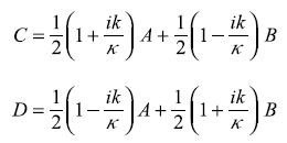
And Eqs (5.83) give

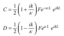
It is easy to see that

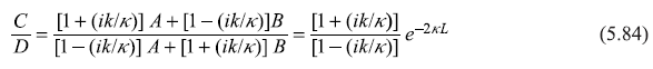
After a little bit of algebra, we get

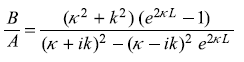
or

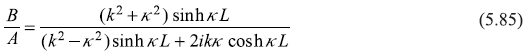
and

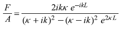
or

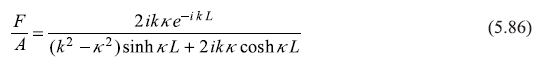
Equations (5.85) and (5.86) will readily lead to the following expressions for the reflection and transmission coefficients:

Equations (5.87) may be put in the following form

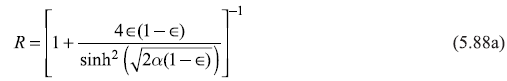
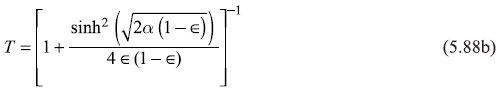
with

and

In writing Equations (5.88), we have used We may easily note that R + T = 1.

As in the case of ‘potential step’ problem for E < V₀, we see finite probability of the particle being found in the region 0<x<L: a purely quantum mechanical effect. This region is totally forbidden for the particle (with energy E<V₀) from the point of view of classical mechanics. Thus, we see, quantum mechanics allows the particle of energy E to penetrate the barrier of potential V₀(>E). The phenomenon is generally called as barrier tunnelling or barrier penetration.

Let us now see how the position probability density |ψ(x)|² looks like in region I, II, and III. We note that as amplitude B of the reflected wave in region I is lesser than that of the incident wave, the resultant wave function ψx)(= Ae^ikx + Be^–ikx) is not zero at any point x in region I. In region III, |ψ(x)|² = |F|² a constant (independent of x). In region II (i.e., inside the barrier), the wave function ψ(x) attenuates as x increases [see Eq. (5.84)]. Therefore, if we plot schematically the position probability density |ψ(x)|² in region I, II, and III, we shall get something like shown in Figure 5.11.

Let us see, qualitatively, how does the transmission coefficient T, given by Eq. (5.88b), vary with energy E of the particle.

1. As E → 0 (i.e., ∊ → 0) Eq. (5.88b) suggests T → 0
2. As E → V₀ (from below)

   (i.e., (1 – ∊) → δ⁺, a small positive quantity)

   

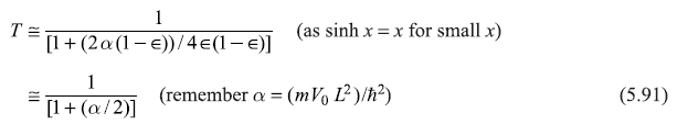
   As the dimensionless numbers α [= (mV₀L²/ħ²)] increases, T decreases. So α may be considered as ‘opacity’ of the barriers.

3. For κL>>1, we can write 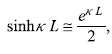so Eq. (5.88b) gives
   

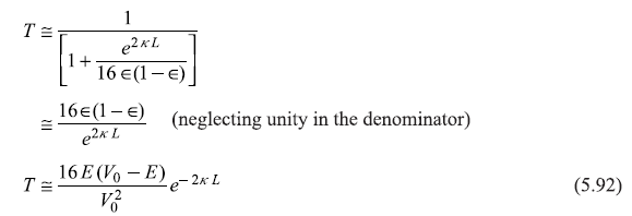
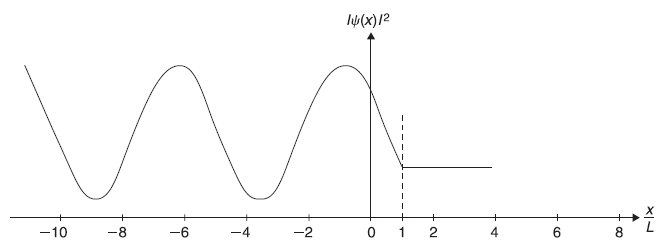
Figure 5.11 Schematic plot of |ψ(x)|² for the case of a rectangular barrier of width L

5.7.2  Case II: E > V₀

For E > V_o, the solution of Schrodinger equation will change only in region II (0 < x < L), where the solution is now given by

 

 

where

 

Again, the conditions that ψ(x) and [dψ (x)/dx] be continuous at points x = 0 and x = L shall give four relations between constants A, B, C, D, and E. Proceeding exactly the same way as that for obtaining the ratios B/A and F/A (for E<V₀ case), we may easily get the expressions for reflection and transmission coefficients as (we have to, in fact, replace κ by ik₁ in equations)

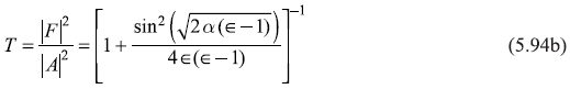
Here we have used We may again note that R + T = 1. In Figure 5.12 we show, schematically, the behaviour of transmission coefficient T as a function of E/V₀, obtained from Eq. (5.88b) for [(E/V₀) < 1], and from Eq. (5.94b) for [(E/V₀) > 1].

We notice the transmission coefficient T is finite (though small) for E < V₀ and, in general, is a bit less than unity for E > V₀. This may be contrasted with the classical mechanical result where T is zero for E < V₀ and T = 1 for E > V₀ (shown in Figure 5.13).

For the quantum mechanical case, we see from Eq. (5.94b) that T = 1 only when

 

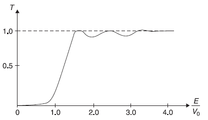
Figure 5.12 Schematic plot of transmission coefficient T as a function of E/V₀ for a rectangular potential barrier

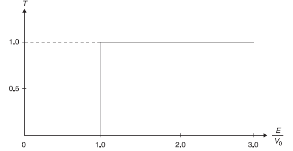
Figure 5.13 Transmission coefficient T (for rectangular barrier) as a function of E/V₀ for classical case

or

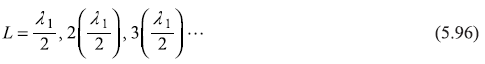
where λ₁= (2π)/k₁ is the de Broglie wavelength in region II. So, T = 1 whenever the barrier width L is an integer multiple of λ₁/2, and, therefore, under such conditions the reflection coefficient is zero. This effect is the consequence of destructive interference between the two reflected waves: one reflected at x = 0 and the other reflected at x = L. In fact, a similar effect has been seen with classical (optical) waves—namely in Fabry-Perot etalon experiment, where a similar interference pattern is observed.

5.8  POTENTIAL WELL OF FINITE DEPTH

Let us consider a rectangular potential well (Figure 5.14) given by

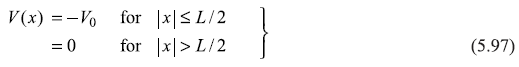
5.8.1  Case I : E < 0

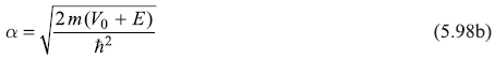
For the energy of the particle in the range –V₀ ≤ E < 0, the particle is confined within the well and hence is in bound state. The Schrodinger equation in region II (i.e., within the well) may be written as

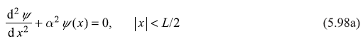
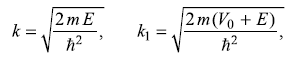
where

Outside the well (i.e., in region I and III), the Schrodinger equation reads

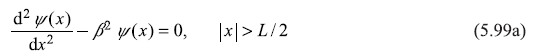
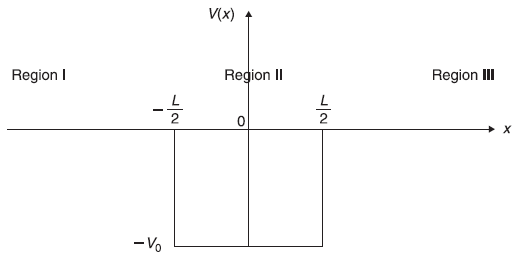
Figure 5.14 A potential well of width L and depth V₀

where

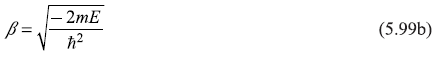
here β is real as E < 0.

Now we note that the potential V(x) [Eq. (5.97)] is symmetric around x = 0; V(−x) = V(x), so the solutions of Schrodinger equations (5.98) and (5.99) are either symmetric or, anti-symmetric in x (see Exercise 5.8). Let us consider the symmetric (i.e., even function) solutions

 

 

 

It may be mentioned here that a term like De^+β|x| has not been added in the wave function in Eq. (5.100b) as it would make the wave function diverge for x → ± ∞: an unphysical situation. The continuity of ψ(x) and at x = L/2 leads to the two equations

From these equations, we get

The anti-symmetric (i.e., odd function) solutions of Eqs (5.98a) and (5.99a), respectively, are,

and

 

 

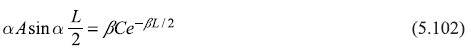
Again, the continuity of ψ(x) and dψ/dx at x=L/2 leads to the transcendental equations

For the given values of m, L, and V₀ the roots of the transcendental equations (5.103) and (5.105) determine the discrete values of E: the energy eigenvalues. These equations may be solved graphically or numerically. For a particular value of energy E, say E_n, we find the ratio A/C [say from Eq. (5.101)]. Hence we find out wave function (say ψ_n) from Eqs (5.100) corresponding to the energy eigenvalue E_n, within a multiplicative constant.

We use here a graphical method to find allowed values of energy E_n. For this, let us introduce two dimensionless quantities ξ = α(L/2) and η = β(L/2). The two equations, Eqs (5.103) and (5.105), which are to be solved (graphically) become

 

 

We may note here that as well as are both positive (E is negative lying in between zero and –V₀; V₀ is positive), and give

So Eqs (5.106) may be written as

and

In Figure 5.15, we plot, schematically, ξ tanξ (solid curves) and –ξ cotξ (dotted curves). We also plot two circles of radii and 5. The points of intersection of these curves with the circles give energy eigenvalues. For a given potential well, the values of V₀ and L are fixed and, therefore, γ is fixed. Let us suppose for a given potential well γ = 5. So, from Figure 5.15 we see, there are four different energy eigenvalues and there would be four corresponding eigenstates. Two eigenvalues E₁ and E₃ correspond to the even solutions (intersection of γ = 5 circle with solid curves) and two values E₂ and E₄ correspond to odd solutions (intersection of the circle with dotted curves). After finding (graphical) solutions of Eqs (5.108) for energy eigenvalues for bound states (E < 0), we may obtain corresponding (normalized) eigenstates from Eqs (5.100) (for even case) and from Eqs (5.104) (for odd case). For the potential well with γ = 5, let us call these wave functions as ψ(x), ψ₂(x), ψ₃(x) and ψ₄(x), respectively. In Figure 5.16, we show schematically the four eigenvalues and corresponding eigenfunctions.

Let us now examine the limiting case of an infinitely deep potential well, that is, the case when V₀→ ∞. In this case γ → ∞ and from Eqs (5.108) we get tan ξ → ∞ which gives

(Note: for n = 0, 2, 4, ... tanξ → ∞ is satisfied while for n = 1, 3, 5, ... cotξ → ∞ is satisfied.)

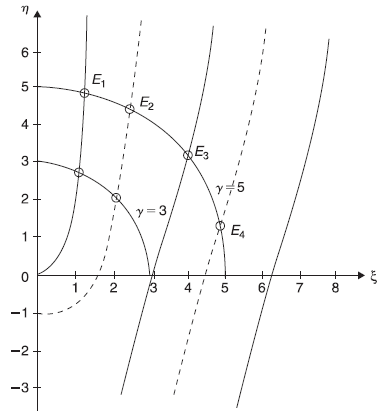
Figure 5.15 Graphical determination of energy levels for a potential well of finite depth. Schematic plot of ξ tanξ (solid curves) and –ξ cotξ (dotted curves). The points of intersection of these curves with the circle of radius γ give the energy levels

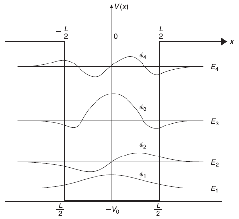
Figure 5.16 Schematic plot of energy eigenvalues and eigenfunctions for a potential well with

or

or

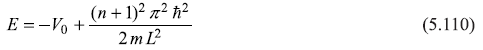
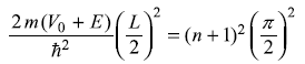
This result is the same as that obtained in Section 5.4 for a potential box (i.e., a potential well of infinite depth). We may note here that E + V₀ [=(n + 1)² π²ħ²/2mL²] is the distance in energy from the bottom of the well and, therefore, represents the kinetic energy of the particle in the well.

5.8.2  Case II : E > 0

We now turn to the case when the particle, in connection with potential well of Figure 5.14 is having positive energy and, therefore, the particle is not bound in the potential well. Considering the particle be incident upon the well from the left, the solutions of the Schrodinger equation in regions I, II, and III, respectively, are given by

 

 

 

 

with

It may be noted that in the region I (x < –L/2), the wave function consists of an incident wave of amplitude A and a reflected wave of amplitude B, while in region III (x > L/2), the wave function consists of only a pure transmitted wave of amplitude C.

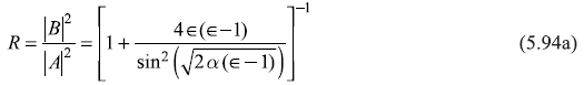
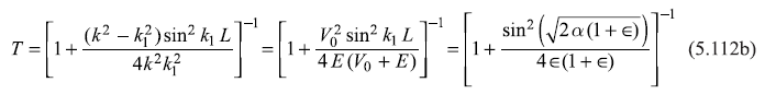
The constants A, B, C, F, and G appearing in Eqs (5.111) can be related by the requirement of the continuity of ψ(x) and dψ/dx at the two boundaries x = ± L/2. We may note that this continuity of ψ(x) and dψ/dx may be realized for any value of E (>0), so all (continuous) values of E (> 0) are allowed energy eigenvalues. Proceeding in the same way as, for example, in Section 5.7, one can solve for the ratios B/A and C/A and one may get expressions of reflection coefficient R = |B/A|² and transmission coefficient T = |C/A|², as

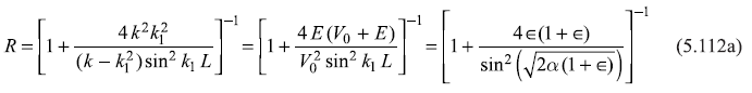
and

with

It may be noted here that if V₀ is replaced in the problem by –V₀, the potential well problem becomes the problem of a potential barrier of barrier height V₀ and width L. The case of potential well of depth V₀ with particle energy E > 0 becomes analogous to the case of potential barrier of height V₀, with particle energy E > V₀. Therefore, it may be easily checked that the expressions for R and T [Eqs (5.112) may be obtained from Eqs (5.94) simply by replacing V₀ by –V₀].

A schematic plot of T as a function of E/V₀ will show similar behaviour as that shown in Figure 5.12.

5.9  KRONIG–PENNEY MODEL

In previous sections, we have studied energy eigenvalues and eigenfunctions of a particle in simple one-dimensional potentials of various forms: potential box, potential well, potential step, and so on. In many cases, we encounter a situation where a particle is moving in a periodic potential. For example, in case of a metal or semiconductor, where the crystal structure is periodic, the electrons experience a periodic potential. So, while discussing the conduction or insulation properties of the solids, we should have the knowledge of what are energy eigenvalues and eigenstates of electrons in the periodic potential of these solids. Let us consider a one-dimensional crystalline solid (say a metal) with positive ions forming a one-dimensional lattice of lattice parameter a (shown in Figure 5.17). The resultant potential of all ions, which an electron feels, is periodic and is shown schematically in the figure. When the electron reaches at the boundary (of the one-dimensional solid), it feels a high potential which gives rise to the work-function of metals.

If we ignore the potential rise at the two boundaries, the potential is periodic throughout and has the property V(x) = V(x + na), here n is an integer. Kronig and Penney suggested a very simple (one-dimensional) potential function which is periodic and has qualitative features of the potential shown in Figure 5.17. This potential, known as Kronig–Penney potential, is shown in Figure 5.18.

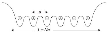
Figure 5.17 Periodic potential in a one-dimensional crystalline solid having N sites

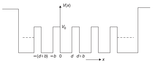
Figure 5.18 The Kronig-Penney potential with periodicity a(= d + b); d being width of the well and b the width of (rectangular) potential barrier of height V_o

To find out energy eigenvalues and eigenstates of a particle in the periodic potential (Figure 5.18), we shall have to solve Schrodinger equation:

with

and

 

 

We notice that the periodic property of V(x) [Eq. (5.115)] may not be realized at the two ends of the lattice. It is a fact that there are a very large number of ion sites in the sample of a one-dimensional solid and, therefore, the effect of potential rise at the two boundaries hardly affects the transport behaviour of the electrons inside. In our treatment of finding eigenstates of electron in potential of Figure 5.18, boundary effects can be avoided if we use periodic boundary conditions (discussed in Section 5.6) on the wave function:

 

 

In fact the use of periodic boundary conditions is one way of getting rid of the effects of the boundaries.

Now the solution ψ(x) of the one-dimensional Schrodinger [Eq. (5.113)] for a periodic potential [Eq. (5.114)], according to Bloch theorem (see Appendix B3), is of the form

 

 

where k is arbitrary (wave vector) and u(x) has the periodicity of the potential V(x), that is,

 

 

Applying the periodic boundary conditions [Eq. (5.116)] on the wave function ψ(x) [Eq. (5.117)], we get

 

 

Comparing Eq. (5.119) with Eq. (5.116), we get

 

or

We now turn to solving Schrodinger equation.

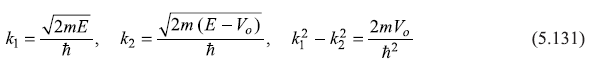
5.9.1  Case-I: E > V_o

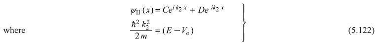
The general solution of Schrodinger equation in the potential well region (0 ≤ x ≤ d) is

The wave function in the barrier region (– b ≤ x ≤ 0) is

The complete solution ψ_I(x) and ψ_II(x) should have the Block form [Eq. (5.117)]. From Bloch theorem

 

 

Now taking x in the interval (–b, 0) (i.e., for –b ≤ x ≤ 0) we have (x + a) lying in the interval (d, a) (i.e., d ≤ x ≤ a), so

 

 

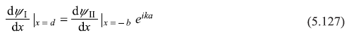
The wave function ψ(x) and its derivative dψ/dx should be continuous at x = 0 and x = d. These boundary conditions should be used to determine the constants A, B, C, and D appearing in Eqs (5.121) and (5.122). Using these conditions at x = 0 give

 

and

 

Condition (5.124) dictates that the wave function at x = d is related with the wave function at x = – b in the following way

 

 

Also their derivatives are related as

These two equations give

The four Eqs (5.125) and (5.128) may be written in the matrix form:

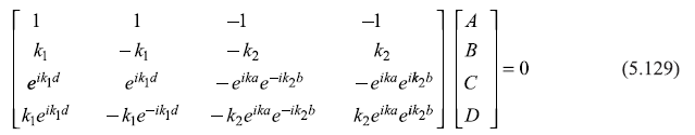
Equation (5.129) has nontrivial solution only if the determinant of the 4 × 4 matrix vanishes. This leads to the following equation (the dispersion relation) as can be checked by doing a bit lengthy but straightforward algebra.

with

5.9.2  Case-II : E < V_o

For the case E < V_o, the general solution of Schrodinger equation in the potential well region remains the same as Eq. (5.121). But in the barrier region the solution takes the form

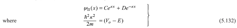
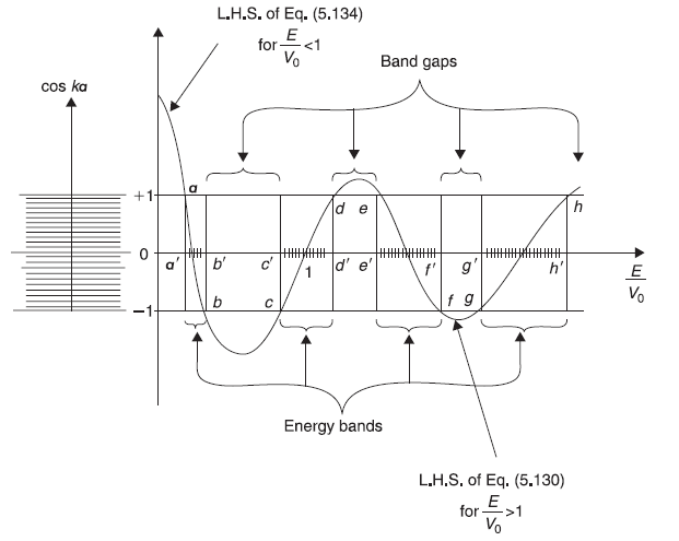
Figure 5.19 Schematic plot of L.H.S. of Eq. (5.134) [for (E/V₀) < 1] and of Eq. (5.130) [for (E/V_o) > 1] as a function of (E/V₀). The two horizontal lines at ordinates +1 and –1 are the two extreme values of R.H.S. of these equations. On the left hand part of the figure we show (schematically) the allowed values of cos ka, where k = k _n= 2nπ/Na Eq. (5.120)

So the dispersion relation for E < V_o case can be easily obtained from Eq. (5.130) simply by the replacement

 

 

The dispersion relation comes out to be

with

Equations (5.130) and (5.134) are transcendental and, therefore, can be solved only numerically to find dispersion relations E(k), that is, to find allowed values of E for given values of wave vectors k. It is obvious that the right hand sides of both Eqs (5.130) and (5.134) have values only within the interval [+1, –1], as |cos k (d + b)| ≤1. So only those values of E are possible for which left hand sides of these equations have values within the interval [+1, –1]. Now it can be easily seen that the function on the right hand side of these equations, that is, cos ka [with allowed values of k as k_n= 2nπ/Na Eq. (5.120)] has only discrete values in the interval [+1, –1]. This aspect is shown on the left part of Figure 5.19, where horizontal lines show, schematically, the allowed values of cos ka. On the right part of Figure 5.19 we show the schematic plot of left hand sides of Eqs (5.130) and (5.134) as a function of E/V₀. The horizontal lines (in the left part of the figure) may be imagined to be extending towards right side and wherever these cut the curve, we get the allowed energy eigenvalues. For example, these lines cut the curve in between the points a and b, c and d, e and f, and so on. So the energy eigenvalues lie in the intervals [a′, b′], [c′, d′],[e′, f′], and so on. These form the allowed energy bands, separated by band gaps. In Figure 5.20, we show schematic plot of allowed energy eigenvalues E as a function of wave vector k, obtained from the graphical solution shown in Figure 5.19.

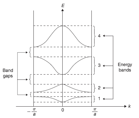
Figure 5.20 Schematic plot of allowed energy eigenvalues E as a function of wave vector k, obtained from the graphical solution shown in Figure 5.19. The energy bands shown as 1, 2, 3, 4 correspond to allowed energy values in the intervals [a′, b′], [c′, d′], [e′, f′] and [g′, h′] respectively of Figure 5.19

EXERCISES

Exercise 5.1

• Consider an electron in a one-dimensional potential box of width L within rigid boundary conditions. Find out ground state energy of electron when L is (i) 1 µm, (ii) 1 nm (iii) 1 Å (iv) 1 fermi.
•  Repeat above exercise for a neutron in the potential box.

Exercise 5.2

Calculate the probability of finding the particle in a one-dimensional potential box of width L, in state ψ_n (with rigid boundary conditions) within the interval and

Exercise 5.3

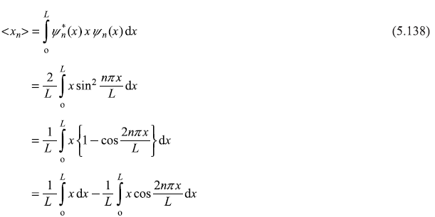
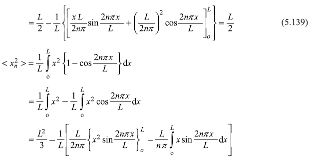
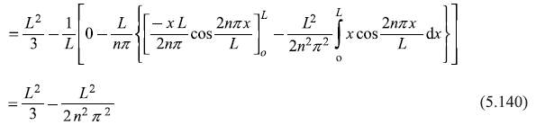
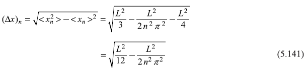
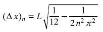
Consider a particle in a one-dimensional box of width L with rigid boundary conditions. Find the expectation values (< x >_n and < x² >_n) of x and x² in n-th state ψ_n. Hence find the uncertainty in the position of the particle in state ψ_n as given by the rms deviation.

Exercise 5.4

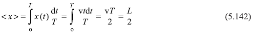
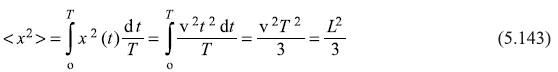
Consider a classical particle moving in a one-dimensional potential box. Find out average value of x and x². Hence find out value of rms deviation of position x and compare it with the corresponding quantum mechanical result of previous exercise.

Exercise 5.5

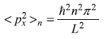
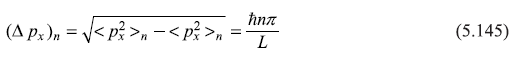
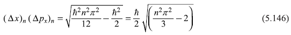
For a particle in a one-dimensional potential box of width L, find the rms deviation (∆ p_x)_n = of linear momentum p_x in state ψ_n. Using the results of Exercise 5.2, find out value of ∆x ∆p_x for n-th state.

Exercise 5.6

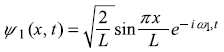
A particle in a one-dimensional box of width L (with RBC) is in a linear superposition state of the ground state and first excited state such that

 

Find out	(a) the position probability density |ψ(x, t)|2
	(b) the average particle position < x (t) >.
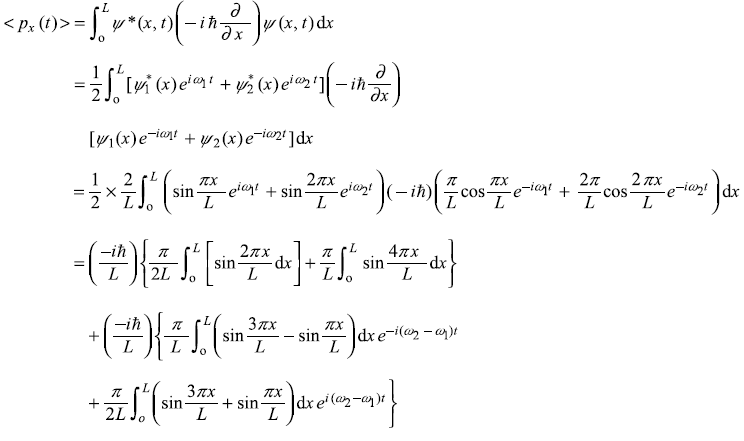
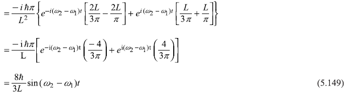
and	(c) the average linear momentum < px(t) >.

Exercise 5.7

Find out energy eigenvalues and eigenstates of a particle in a one-dimensional box of width L (with RBC) extending from x = –L/2 to x = L/2.

Exercise 5.8

The potential box in Exercise 5.7 has the property V(– x) = V(x), the so-called inversion symmetry. Discuss, what restriction does this property (of inversion symmetry) of the potential puts on the wave functions of the particle?

Exercise 5.9

Consider a one-dimensional potential well in the form of a delta function V(x) = – A δ(x). Show that there is only one bound state of the particle. Find energy eigenvalue and eigenstate.

Exercise 5.10

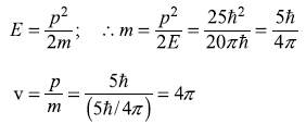
A free particle moving in x – direction has time-dependent wave function

What are the value of (i) wavelength, (ii) linear momentum, (iii) mass, (iv) velocity of the particle, and (v) total (kinetic) energy?

Exercise 5.11

What is the probability current density of the particle with the wave function given in Exercise (5.10)?

Exercise 5.12

Consider following functions of position x. Test, which of these are the eigenstates of (i) the linear momentum operator (ii) the square of linear momentum operator

• A sin kx
•  A cos kx
•  A (sin kx + cos kx)
•  A x²
•  A(x² + b²)
•  A e^–αx2
•  A e^ikx
•  A e^–ikx

Exercise 5.13

A beam of electrons is incident from left, normally, on a semi-infinite step-potential (Figure 5.5) 5.0 eV in height. The incident electrons have kinetic energy E (when to the left of the step-potential). What is the relative probability that any given electron will be reflected back by the step-potential, when

• E = 5.02 eV
• E = 10.0 eV
• E = 4.98 eV

Exercise 5.14

A beam of electrons having speeds of 10⁶ m/s in field-free space is incident from left, normally, on a semi-infinite step-potential 3.0 eV in height. The step barrier begins at x = 0. The electron probability density P(x) = |ψ(x)|² is given as 1000 electrons/cm³ in the incident beam. Find electron probability density P(x) within the barrier at

•  x = 10 Å
• x = 50 Å

Exercise 5.15

In the above exercise, compute the total probability of finding an electron in the regions.

• 0 < x < 10 Å
• 10 Å < x < 50 Å
• 50 Å < x < ∞

SOLUTIONS

Solution 5.1

1. Ground state energy of electron is
   
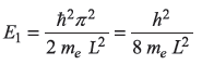
   • For L = 1µm,
     
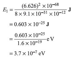
   • For L = 1 n m,        E₁ = .37 eV
   • For L = Å,         E₁ = 37.0 eV
   • For L = 1 fm,         E₁ = 37 × 10⁴ M eV = 370 G eV
2. For neutron
   •  For L = µm,        E_l = 2.01 × 10^–10 eV
   •  For L = 1 nm,        E₁= 2.01 × 10^–4 eV
   • For L = 1 Å,        E₁= 2.01 × 10^–2 eV
   •  For L = 1 fm,        E₁ = 2.01 × 10² M eV

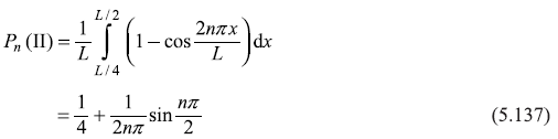
Solution 5.2

Let us denote the two probabilities in the intervals and as P_n(I) and P_n(II), respectively. Then

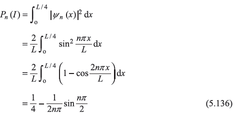
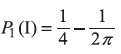
For n = 1,

For n = 2,

For n = 3,

Now

For n = 1,

For n = 2,

For n = 3,

Solution 5.3

∴

Solution 5.4

Let a classical particle be moving with speed v in the potential box of width L. Let the particle start at t = 0 from one end of the well, then it reaches the other end in time T = (L)/v (and shall go on transversing the well in every T time). The average value of the position is given by

Similarly, average values of x² is

Solution 5.5

From Eq. (5.44) we have

 

∴

From Eq. (5.141) we have

∴

Solution 5.6

(a)

where

and

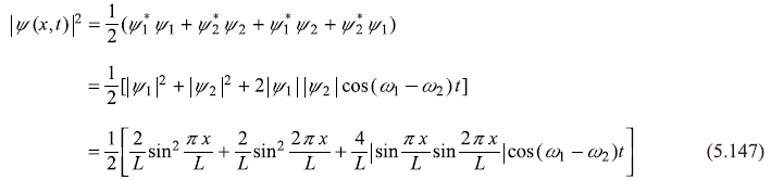
The resultant probability density |ψ(x, t)|² has an oscillatory behaviour as a function of time. It oscillates between two probability densities and sinusoidally with frequency (ω₂ – ω₁) = (3π² ħ)/2mL².

 

(b)

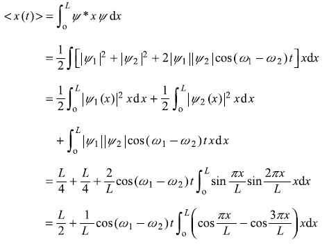
After integrating the integral in second term by parts, we get

(c)

Solution 5.7

The Schrodinger equation given by Eq. (5.26) is to be solved for the potential V(x) given by

 

Let the general solution be

 

 

The arbitrary constants A and B are determined by using the boundary conditions.

We get

and

From these equations, we get

 

 

∴

 

 

Let us take

 

 

Then

∴

or

or

For

 

 

we get

∴

or

or

So normalized wave functions are

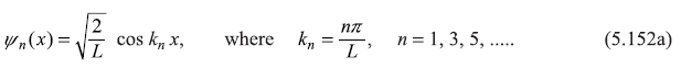
and

The energy eigenvalues are

Solution 5.8

In Exercise 5.7, the potential is symmetric about x = 0, so has the property V(–x) = V(x). Any other potential, which is an even function of x [say harmonic potential has this property (of inversion symmetry). The Schrodinger equation for such potential V(x) is

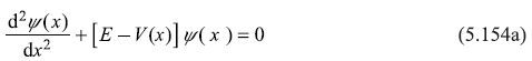
Let us substitute

 

 

we get

Here we used the symmetry property of the potential; V(–x′) = V(x′). Now in Eq. (5.154b), x′ is space variable and we may write any variable in its place, say x.

So, Eq. (5.154b) is nothing but

Comparing Eqs. (5.154 a) and (5.154 c), it is clear that if ψ(x) is an eigenfunction of the particle [in potential V(x)], then ψ(–x) is also an eigenfunction in V(x). So, if the state in non-degenerate, the two wave functions ψ(x) and ψ(–x) must be linearly dependent; ψ(–x) must be some multiple of ψ(x).

 

 

If the transformation x → –x is made again in Eq. (5.155), we get

 

or

 

Hence,

 

 

The eigenfunctions having the property ψ(–x) = ψ(x) are said to have even parity and those with the property ψ(–x) = – ψ(–x) to have odd parity. So, all wave functions (for bound states) of a particle, in a symmetric potential, are either even or odd functions of x.

Solution 5.9

The Schrodinger equation for the given delta function potential is

For x < 0 and x > 0, the equation becomes

where

We are interested in solving Eq. (5.157) for negative values of energy E, so κ² in Eq. (5.158) is a positive quantity. The corresponding wave function should vanish for x → ∞ as well as x → –∞. So the solution of Eq. (5.157) should be

 

 

Let us integrate Eq. (5.157) from x = –∊ to x = ∊ (∊ being infinitesimal quantity). We get

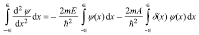
It is clear from Eqs. (5.159) that ψ(x) is continuous at x = 0, therefore, the first term on R.H.S. of above equation vanishes. So we get (using the properties of delta function).

Now from Eqs (5.159) we have

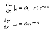
So

 

From Eqs (5.160) and (5.161), we get

Therefore,

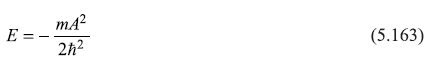
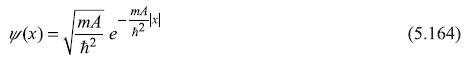
The corresponding wave function (5.159) can be easily obtained in normalized form to be

Solution 5.10

Let us compare the given wave function with the standard form

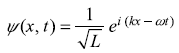
We get

 

∴

 

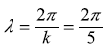
so that the kinetic energy E is

 

Now

Solution 5.11

Solution 5.12

A function f(x) is the eigenfunction of an operator Ŝ if an eigenvalue equation is satisfied, for example,

 

 

where operator Ŝ operating on f(x) gives eigenvalue s. Let us now check the given functions by operating operator [– iħ(d/dx)] and [– ħ² (d²/dx²)] on these

• •  
    
    = –iħ Ak cos kx     (No)
  •  
    
    = ħ²k² A sin kx (Yes)
• •  
    
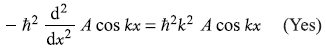
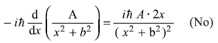
    = iħ Ak sin kx     (No)
  •  
    
• •  
    

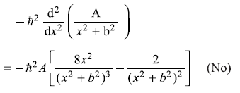
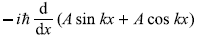
    = –iħk (A cos kx – A sin kx)      (No)

  •  
    
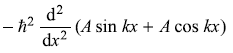    = –ħ²k² (A sin kx + A cos kx)    (Yes)
• •  
    
  •  
    
• •  
    
  •  
    
• •  
    
  •  
    
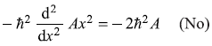
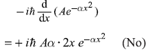
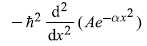    = 2Aħ²αe^–αx2 [1 – 2αx²]    (No)
• •  
    
  •  
    
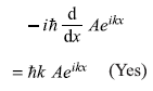
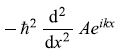    = ħ²k² Ae^ikx    (Yes)
• •  
    
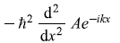
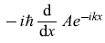    = –ħk Ae^–ikx    (Yes)
  •  
    

Solution 5.13

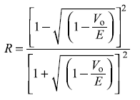
• The reflection coefficient is given by Eq. (5.78a)
  

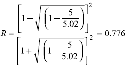
  for V_o = 5.0, E = 5.02 eV, we have

  
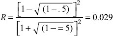
•  For        E = 10.0 eV
  
• For        E = 4.98 eV (i.e., E < V_o)
  R = 1.0

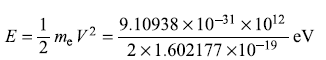
Solution 5.14

Energy of the incident electrons

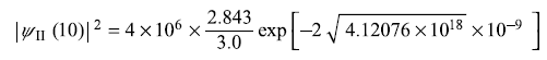
From Eq. (5.69b), we have

where and k² and κ² are given by Eqs (5.63). We get

So

Here 

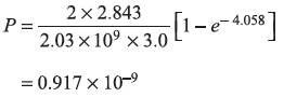
(a)   

so

 

(b)

 

 

Solution 5.15

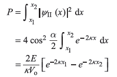
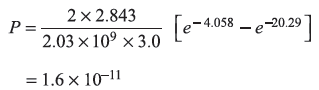
To find probability, we shall take A² = 1. The probability of finding the electron in between x₁ and x₂ is

•  
  
•  
  
•  
  

REFERENCES

1. Bransden, B.H. and Joachain, C.J. 2000. Quantum Mechanics. Singapore, Pearson Education Ltd.
2.  Schiff, L. 1968. Quantum Mechanics. 3rd edn., New York, NY: Mc-Graw Hill.
3. Levi, A.F.J. 2003. Applied Quantum Mechanics. Cambridge, Massachusetts: Cambridge University Press.
4.  Fromhold Jr, A.T. 1981. Quantum Mechanics for Applied Physics and Engineering. New York, NY: Academic Press.
5. Liboff, R.L. 1992. Introductory Quantum Mechanics. Reading, Massachusetts: Addison-Wesley.
6.  Kittel, C. 2005. Introduction to Solid State Physics 7th edn., New York, NY: John Wiley and Sons.
7. Ashcroft, N.W. and Mermin, N.D. 2001. Solid State Physics. Singapore: Harcourt College Publishers.