Chapter 2

Wave-particle Duality

The opposite of a profound truth may well be another profound truth.

—Niels Bohr

2.1   INTRODUCTION

In this chapter we shall discuss, in brief, various experiments which have been performed to investigate the nature of microscopic objects like electrons, neutrons, and electromagnetic radiations. There are experiments, such as Young’s two-slit experiment and X-ray diffraction experiment, which suggest that electromagnetic radiations propagate in the form of waves. On the other hand, there are experiments, such as photoelectric effect and Compton scattering, which suggest that electromagnetic radiations consist of particles in the form of quanta of energy having well-defined linear momentum, well-defined energy, and so on. The same is true about the matter particles, such as electrons, protons, and neutrons. There are experiments, such as electron diffraction and neutron diffraction, which suggest that electrons in the electron beam or neutrons in the neutron beam propagate in the form of waves having well-defined wavelength.

2.2   YOUNG’S TWO-SLIT EXPERIMENT

Let us revisit briefly Young’s two-slit experiment which shows that light travels in the form of waves. In Figure 2.1, S is the source of monochromatic light. S₁ and S₂ are two narrow slits in an opaque plane surface. S is put symmetrically in front of S₁ and S₂ . On the other side of the slits is a screen placed parallel to the opaque surface having S₁ and S₂ . One observes a light intensity variation, with maxima and minima on the screen (as shown in Figure 2.1), which can be explained only if one assumes that light propagates in the form of waves.

We proceed now to analyse Young’s experiment quantitatively. Let us assume S as the source of light waves of single wavelength λ only. S₁ and S₂ shall now act as two coherent sources. Let us consider an arbitrary point P on line AB on the screen. The light waves from S₁ and S₂ will superpose on reaching P. For getting maxima at P, the condition

 

 

must be satisfied. Now with the information given in Figure 2.1, we get

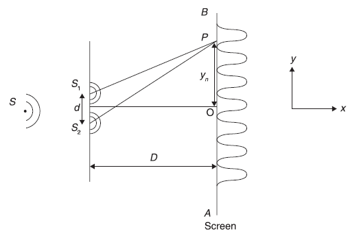
Figure 2.1 Young’s two-slit experiment

From Eqs (2.1) and (2.2), we get

The separation between two successive maxima, called the fringe width, is obtained as

 

 

An expression for the resultant intensity variation on the screen along y direction may be obtained as follows.

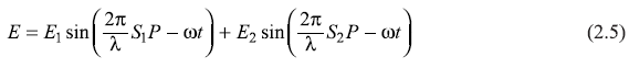
S is the source of monochromatic light of wavelength λ and (angular) frequency ω. Let E₁ and E₂ be the (electric field) amplitudes of light waves reaching P from S₁ and S₂, respectively. According to the principle of superposition (of waves), the resultant amplitude E of the field at P is

The light intensity I at P is proportional to E²,

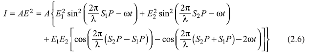
where

represents the phase difference between the two waves arriving at point P from S₁ and S₂. In writing Eq. (2.7), we have considered the time average of functions sin² and sin² and have replaced these by 1/2. As point P moves on the screen along y-axis, the phase difference δ changes and so does the intensity I of the resultant wave. The intensity I varies between the maxima and minima this is really what has been observed experimentally.

2.3   BRAGG’S X-RAY DIFFRACTION

X-rays are electromagnetic radiations. If X-rays propagate in the form of waves like light waves, these shall exhibit interference and diffraction phenomenon. It has been observed that when X-rays fall on a crystalline solid, the solid works as a three-dimensional grating and produces diffraction pattern. Actually, ordinary devices like ruled diffraction gratings do not produce any observable diffraction effects with X-rays. In short, in this chapter, we describe Bragg’s X-ray diffraction law. In this experiment, monochromatic X-rays are incident on a crystalline solid. The X-rays are diffracted in a number of selected directions. In fact, the diffraction pattern obtained on the flat film consists of a central spot and a definite pattern of spots around the central spot. W. L. Bragg gave a simple explanation of the diffraction pattern, called Bragg’s diffraction law. According to Bragg, the X-rays incident on a crystal are scattered by the atoms (ions) of the crystal, in all possible directions. These atoms (ions) are arranged in a regular fashion in the crystal, and, therefore, the scattered waves interfere constructively in some directions and destructively in other directions. The directions of constructive interference (and hence of maximum intensity of X-rays) may be obtained, following Bragg, by assuming the solid as consisting of a set of parallel atomic planes. In Figure 2.3, different sets of parallel planes are shown (only two-dimensional counterpart is shown, where set of parallel lines represent the set of parallel planes in real solid). According to Bragg, the maxima are produced due to the reflection of the incident X-rays from the various sets of parallel planes, called Bragg planes.

Let us consider an X-ray beam of wavelength λ incident upon a crystal at an angle θ with respect to a set of Bragg planes with spacing d (Figure 2.2). The parallel rays AC and BD are reflected from plane I and II, respectively, at atoms C and D in directions CE and DF. Let CP and CQ be the two perpendiculars drawn from C on directions BD and DF, respectively. The two reflected rays will be in phase, if the path difference between these rays (i.e. PD + DQ) is an integer multiple of λ. From Figure 2.2, PD = DQ = d sin θ. Hence, the condition of maxima becomes

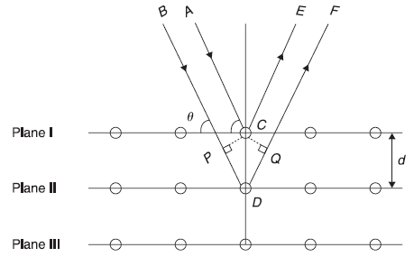
Figure 2.2 Bragg reflection from a family of lattice planes in a crystal

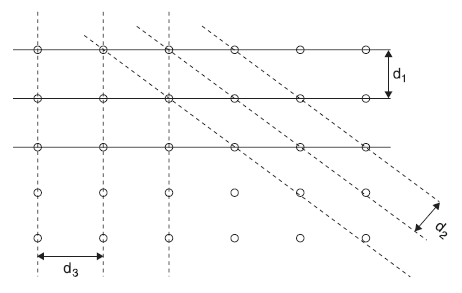
Figure 2.3 Different sets of parallel planes with spacing d₁, d₂, and d₃

 

where n = 1, 2, 3, … correspond to the first-, second, and third-order maxima, respectively. Equation (2.9) is known as Bragg’s law. The experimentally observed X-ray diffraction patterns can easily be explained on the basis of Bragg’s law.

2.4   PHOTOELECTRIC EFFECT

After discussing two experiments, the double-slit experiment and X-ray diffraction experiment, which suggest that the electromagnetic radiations propagate in the form of waves, we shall now discuss an experiment of photoelectric effect which suggests that the electromagnetic radiations consist of particles in the form of quanta of energy and definitely not in the form of waves.

The apparatus for the study of photoelectric effect consists of a vacuum chamber containing metallic plate P and a collector C [as shown in Figure 2.4(a)]. A voltage V is applied between the plate and the collector, and a beam of ultraviolet light is incident on the plate. Some of the photoelectrons emitted from the plate shall reach the collector, thus forming the photoelectrons current. When collector is at the positive potential, almost all photoelectrons emitted from the plate shall reach the collector. As collector potential is made negative, photoelectron current decreases. The variation of photoelectron current with collector potential for different intensities of light of a fixed frequency is shown in Figure 2.4(b). Figure 2.4(c) shows the variation of photoelectron current with collector potential for different frequencies of radiations. All the experimental results may be summarized as follows:

1. The emission of photoelectrons takes place almost instantaneously with the arrival of light beam on the metal surface.
2. For a given metal plate, there is a minimum cut-off frequency v₀ (called the threshold frequency), below which no photoelectrons are emitted irrespective of the intensity of light.
3. For a given frequency of light, as the collector potential is increased negatively, the photoelectron current decreases and becomes zero at a definite negative potential V₀ (called the stopping potential) of the collector. Furthermore, the stopping potential increases linearly with the frequency of the incident radiation. However, the stopping potential is independent of the intensity of the radiation beam.
4. For a given metal plate and radiation frequency, the photoelectron current, including the saturation current, is found to increase linearly with the intensity of the radiation beam.

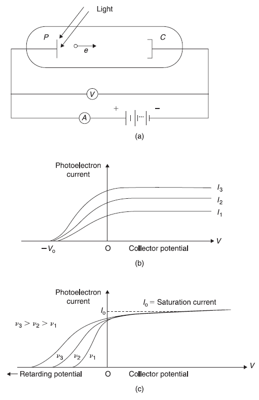
Figure 2.4 Photoelectric effect: (a) Experimental arrangement (b) Variation of photoelectron current with collector potential for different radiation intensities (c) Variation of photoelectron current with collector potential for different frequencies of radiation

The wave theory of light is not able to explain many of the observed facts. For example, consider the maximum kinetic energy K_max of photoelectrons. K_max = eV₀ is fixed for a particular frequency of radiation beam [see Figure 2.4 (b)]. However, on the basis of wave picture of electromagnetic radiations, the force which radiation exerts on the electrons in the metal should be proportional to the magnitude of the electric vector E of the incident radiation beam. This suggests that K_max should depend on beam intensity, contrary to experimental observations. Similarly, observation of a threshold frequency v₀ cannot be understood on the basis of wave picture of radiations, as an intense beam of frequency lesser than v₀ should have enough energy to be imparted to electrons in the metal to be ejected out.

Einstein was able to explain all the experimental observations by proposing that electromagnetic radiations consist of small packets, the quanta of energy, called photons. According to Einstein, each photon of electromagnetic radiation of frequency v has energy E given by

 

 

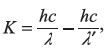
where h is the Planck’s constant. According to Einstein, in the photoelectric effect experiment, an electron (of metal) absorbs a quantum of energy hv of the incident radiation. When the energy hv absorbed by the electron exceeds the required minimum energy ϕ for the electron to be liberated from metal, the electron comes out of metal with kinetic energy K given by

 

 

The maximum kinetic energy K_max is acquired by the electron having minimum value of ϕ (say ϕ₀ which is called the work function of the metal). Thus,

 

2.5   COMPTON EFFECT

The Compton effect experiment gives direct evidence that electromagnetic radiations consist of photons, which collide with electrons, for example, like one billiard ball colliding with other ball. In Figure 2.5, we show, schematically, the experimental arrangement of Compton effect. An X-ray beam of known single wavelength from source S falls on the metallic foil and gets scattered in various directions. The wavelengths of scattered X-rays are determined at various angles ϕ by X-ray spectrometer.

In this experiment, Compton found that the X-rays scattered through a given angle ϕ actually consist of mainly two components: one has the same wavelength as that of incident X-rays, and the other has wavelength shifted on higher side relative to the incident wavelength by an amount that depends on the angle ϕ.

Compton was able to explain the experimental results by treating the X-ray beam as a beam of photons, each of energy hv and linear momentum hv/c individually colliding with the electrons of foil. Let us consider a photon of energy hv and linear momentum p (= hv/c) incident along x-axis on an electron at rest in the laboratory coordinate system. After the collision, the photon shall be scattered in one direction and the electron will recoil in some other direction. Let the photon be scattered in a direction making an angle ϕ with x-axis and the electron recoiled at an angle θ from x-axis (as shown in Figure 2.6). In fact, the scattered photon is not the same as the incident photon. The incident photon shall lose some amount of energy to electron, and, therefore, its energy hv′ is less than the energy hv of incident photon. Thus, the process really involves two different photons.

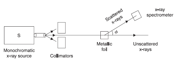
Figure 2.5 Compton effect experiment

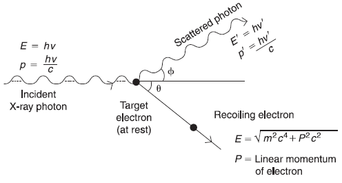
Figure 2.6 Kinematics of photon-electron collision in Compton effect

Now conservation of linear momentum says

 

 

where p′ [= (hv′ /c)] is the linear momentum of the scattered photon and P is the linear momentum of the recoiled electron. Equation (2.13) gives

 

 

and the conservation of energy gives

where m is its rest mass of the electron. Equation (2.14) may be written as

or

 

 

Now we have from Eq. (2.15)

 

 

Thus, from Eqs (2.16) and (2.17), we get

 

 

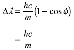
or

which gives us the Compton shift. The quantity h/mc is known as the Compton wavelength of the particle (electron in the present case). For electrons h/mc = 2.43 × 10^–12 m = 2.43 × 10^–2 Å.

2.6   WAVE-PARTICLE NATURE OF ELECTROMAGNETIC RADIATIONS

In Sections 2.2 and 2.3, it was observed through Young’s two-slit experiment and X-ray diffraction experiment that electromagnetic radiations show phenomenon of superposition of waves through interference and diffraction patterns. Therefore, it can be concluded that, without any doubt, radiations propagate in the form of waves. On the other hand, in Sections 2.4 and 2.5, through the photoelectric effect experiment and the Compton effect experiment, it becomes clear that radiations consist of particles called photons.

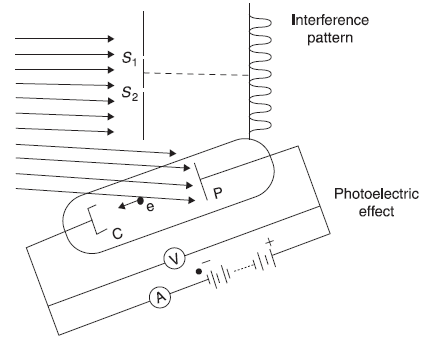
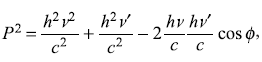
Figure 2.7 Wave and particle nature of radiations

Figure 2.7 shows an extended beam of radiations from a monochromatic source. One part of the beam falls on two-slit arrangement and produces fringe pattern. The other part of the same beam falls on the metallic plate P of the photoelectric apparatus, which as we have seen in Sections 2.4, suggests particle nature of radiations. It is surprising to see that the same beam when interacting with two-slit arrangement compels us to believe in its wave nature, while it compels us for its particle nature when it interacts with electrons in the metallic plate. It seems the nature has not done justice with us by creating the conflicting situations. Well, before we try to analyse the situation further, let us discuss more unexpected experimental observations in the next section.

2.7   ELECTRON/NEUTRON DIFFRACTION

In this section, let us discuss some experiments with what we generally perceive as matter particles such as electrons, protons, and neutrons. Electrons and protons, for example, are perceived to have well-defined charge and mass, in the so-called Mullikan’s experiment. Never, in any experiment, an electron has been observed with fractional charge or mass. The picture in our mind of an electron or proton is that it is a tiny particle like a very small, (spherical) ball with definite charge and mass. Let us try to see what an electron or proton looks like if we probe it more closely. In this context, we propose the following experiment.

Let us consider monoenergetic beam of electrons, obtained from a heated filament, propagating in positive x-direction and falling on a screen having two narrow slits S₁ and S₂. Let us first consider these electrons to propagate like very small balls. Let the flux of beam (number of electrons crossing unit area per unit time) be very small so that the electrons are away from each other and not to influence each other through Coulomb interaction. In front of the two-slit system is a screen D (in y–z plane) having detectors D₁, D₂, … fixed along y-axis (Figure 2.8).

When slit S₁ is open (and S₂ closed), the electrons which are detected by detectors on D are those which pass through S₁ either unhindered or scattered by the edges of S₁ in various directions. If we plot the number of electrons N₁, N₂, … reaching at various detectors D₁, D₂, … as a function of their positions y₁, y₂, …, we shall obtain a curve similar to that shown as I₁ in Figure 2.8(a). The shape of the curve is not important. Main characteristic of the plot shall remain: it shows maxima in front of S₁ and decreases rapidly on both sides. Similarly, plot I₂ can be obtained when S₁ in closed and S₂ is open. When both S₁ and S₂ are open, one simply expects to obtain the result I, which is the sum of I₁ and I₂.

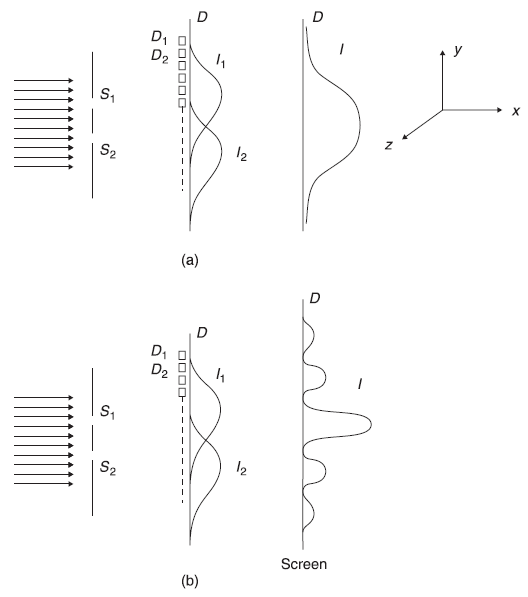
Figure 2.8 Two-slit experiment (a) with beam of particles (b) with beam of waves

Now imagine for a moment that electrons instead of propagating like particles were propagating like plane waves in the two-slit experiment. Well, it may not be clear at the moment why should we imagine the electrons to behave like this, but let us do it for the moment. Hence, it simply becomes the case like that of a two-slit interference experiment. When slit S₁ is open, the electrons in the form of waves shall pass through S₁. The wave passing through S₁ shall produce single (narrow) slit diffraction pattern. The detectors D₁, D₂, ... shall detect the number of electrons N₁, N₂, … reaching there. Again, we plot the number of electrons reaching y₁, y₂, … and will find a curve shown as I₁ in Figure 2.8(b). Similarly, when S₂ is open (and S₁ closed) one finds a curve I₂. When both the slits are open, we expect a two-slit interference pattern, that is, we expect that when N₁, N₂, … are plotted as a function of y₁, y₂, … one should obtain fringes as shown by curve I. If the electrons are propagating in the form of waves, these waves, after passing through slits S₁ and S₂, should superpose (with different phase difference at different position y), just like ordinary waves, on the screen and should show interference pattern.

Should we now not go to the actual experiments done with the electron beam? Well, strictly speaking two-slit experiment has never been done in reality with electron beam. But, whatever experiments with electron beam have been done (and these are the experiments of electron beam with arrays of slits in three dimensions—the Davisson and Germer experiment of electron diffraction with solids; refer to Section 2.8) have confirmed that the observed intensity pattern of electrons on the screen, after passing through two-slit arrangement, is exactly like pattern I shown in Figure 2.8(b) and not like pattern I as shown in Figure 2.8(a). In fact, in the simplified description of the two-slit diffraction experiment, we may say, one measures the number of electrons N₁ reaching a small region around position y₁ on the screen with the detector D₁ at that place. Similarly, N₂ around y₂ with detector D₂ and so on are measured. Now when one plots N₁, N₂, N₃, … as function of y₁, y₂, y₃, …, one finds exactly the same pattern as that obtained by plotting the resultant intensity I (which is proportional to the square of resultant wave amplitude).

2.8   DAVISSON AND GERMER ELECTRON DIFFRACTION EXPERIMENT

In 1927, C. Davisson and L. Germer, through their experiment of electron diffraction with single crystal, confirmed that electrons in the electron beam propagate like waves. Davisson and Germer used an apparatus, as sketched in Figure 2.9(a), where a monoenergetic beam of electrons from the electron gun is incident on a single crystal of Ni and the scattered beam is detected by electron detector. The energy and direction of the incident beam and the position of the detector vary. The number of electrons N scattered at an angle θ to the incident direction was measured by the electron detector. The data obtained for electron beam of energy 54 eV is shown schematically in Figure 2.9(b). The intensity of the scattered electrons is maximum for θ = 0, decreases as θ increases with a minimum near θ = 35° and is again maximum near θ = 50°. While the strong scattering at θ = 0 may be easily explained using both particle and wave theory, the minima at 35° and the peak at 50° can only be explained using the wave theory. It is, respectively, the destructive and constructive interference of the electron waves scattered by the regular crystal lattice (which is behaving just like a three-dimensional grating for the electron waves) which gives minima near θ = 35° and maxima near θ = 50°.

Referring to Figure 2.9(c), the constructive interference occurs when the Bragg condition

 

 

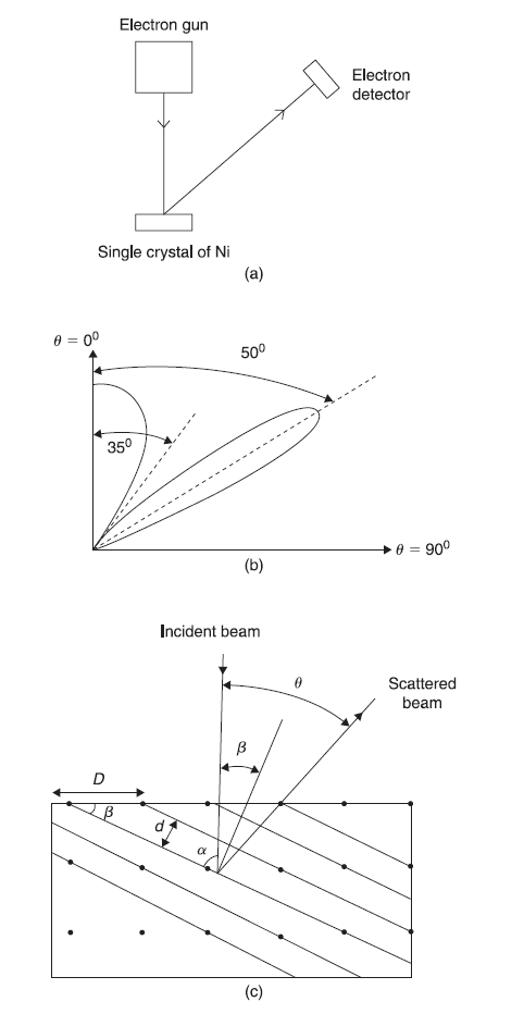
Figure 2.9 (a) Schematic sketch of electron diffraction experiment of Davisson and Germer (b) Plot of scattered intensity I (θ) as a function of scattering angle θ, of 54 eV electrons (c) Scattering of electron waves by a crystal according to Bragg’s law

is satisfied, where d is the spacing of the Bragg planes [indicated in the Figure 2.9(c)]. From the figure, we have

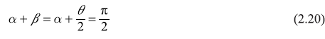
and

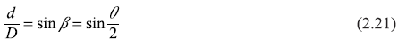
From Eqs (2.19) and (2.20), we have

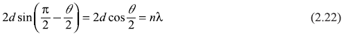
Hence,

or

 

 

Let us find out the wavelength λ of electron waves from Eq. (2.23). The X-ray diffraction experiments on Ni single crystals give the atomic spacing D = 2.15 Å. Let us assume the peak at θ = 50° corresponds to first-order diffraction (n = 1). Therefore, we get λ = 2.15 sin 50° = 1.65 Å. On the other hand, the de Broglie wavelength of an electron of kinetic energy 54 eV comes out to be [see Eq. (3.16d)]

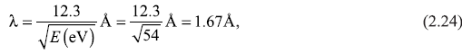
which agrees with the above-mentioned value 1.65 Å within experimental error. Davisson and German did experiment for various values of energy E of incident beam. For each case, the value of wavelength found experimentally [Eq. (2.23)] matched with the de Broglie wavelength found from Eq. (2.24).

2.9   WAVE-PARTICLE NATURE OF MATTER

In Sections 2.2 to 2.6, we saw that electromagnetic radiations manifest themselves in two different ways; behave like waves in one set of experiments and like particles in another set of experiments. Now, as we saw in Sections 2.7 and 2.8, a similar situation is there with matter particles too. Matter particles when detected (in a detector) always show particle nature: well-defined position, mass, charge, and so on. While when the same particles, in the form of particle beam, meet two-slit arrangement or three-dimensional grating, show diffraction pattern–a characteristic of waves. So just like electromagnetic radiations, which show wave or particle nature depending upon the type of experiment we choose; a system of matter particles also show wave or particle nature, again depending upon the type of experiment we choose.

2.10   WHAT IS THE REAL NATURE OF MATTER AND RADIATIONS?

Physics is really the study of the behaviour of physical systems (matter and radiations), both at macroscopic and at microscopic levels, under various conditions. Tremendous progress had been made in the study of nature of physical systems at macroscopic level during the nineteenth century. Thereafter, it was the turn of studying nature of matter and radiations at microscopic level, which started at the beginning of twentieth century. But, as we have seen in previous sections, soon it became evident that the real nature of matter and radiations at microscopic level is not at all clear; both the radiations and matter show wave nature as well as particle nature depending upon the experimental setup one chooses to probe their nature. It seems to be a disturbing situation.

Let us revisit the electron two-slit interference experiment [Figure 2.8(b)], The variation of the resultant intensity I, when both slits S₁ and S₂ are open is characteristic of two-slit diffraction pattern, and it confirms the electrons propagating in the form of waves. The electron wave divides itself into two parts at S₁ and S₂ (like what light wave does in Young’s two-slit experiment) and recombine at different positions on the screen with different values of phase differences and, therefore, giving rise to different amplitudes (intensities). Let us imagine this experiment is done with an electron beam such that only one electron is sent to the slit system at a time. The electron passes through the slit system, reaches the screen and is detected by one of the detectors there, then the second electron is sent, and so on. When a large number of electrons have been sent, one plots the number of electrons detected by various detectors as a function of their position y. Surprisingly, the pattern obtained is the same as that with an intense beam of electrons. This simply means that in this experiment even a single electron was propagating in the form of a wave which encounters two slits, divides itself into two parts, recombines on the screen, and gets detected by one of the detectors as a whole single electron. This is all what is concluded from the two-slit diffraction experiment.

Similar results have been obtained with Young’s two-slit experiment with light. Here, the intensity of light incident on slit system is made smallest possible such that only one photon is incident at a time. The experiment with such a low-intensity light was done for a long duration. The accumulated light energy I on the screen was found to have the same pattern as that in the usual two-slit experiment. It again suggests that a single photon, incident on a two-slit system, was propagating in the form of a wave, dividing itself into two parts at S₁ and S₂ and then recombining on the screen.

Therefore, irrespective of the intensity of the light beam (and of number of electrons in the electron beam), both the light and electron beams show wave nature when interacting with the two-slit arrangement. Moreover, the same light beam (and electron beam) show particle nature when experiments such as photoelectric effect or Compton effect (e/m determination Mullikan experiment) are performed.

The above explanation seems to suggest that it depends in a way upon the wishes of the experimentalist, which equipment, two-slit arrangement or photoelectric effect setup, he/she chooses to find out the nature of radiations. If the observer chooses one equipment, he/she ‘sees’ radiations behaving like waves, while if he/she chooses the other equipment, he/she ‘sees’ radiations behaving like (photon) particles. Should it depend upon the observer to conclude about ‘what is the nature of microscopic entities?’ Are things so arbitrary at microscopic level?

The situation is really uncomfortable for a common man who generally believes in the doctrine of ‘realism’. This doctrine admits the existence of ‘things’ independent of our own existence. The ‘things’ or objects of ordinary size are not affected by the mere action of observation, and the same is expected to be true for very large (e.g., satellites and planets) as well as very small (e.g., molecules and atoms) objects. In fact, the concept of reality is so deeply ingrained from our very childhood that we generally are not ready to rethink on this issue. ‘Things are as they are even if we do not look at them and even if we do not understand them’ is the philosophy of a common man. As R. P. Feynman states,

‘... If a tree falls in a forest and there is nobody there to hear it, does it make a noise? A real tree falling in a real forest makes a sound, of course even if nobody is there. Even if no one is present to hear it, there are other traces left. The sound will shake some leaves, and if we were careful enough we might find somewhere that some thorn had rubbed against a leaf and made a tiny scratch that could not explain unless we assumed the leaf was vibrating. So in a certain sense we would have to admit that there is a sound made.’

The two opposite pictures of wave and particle of radiation and matter found in so different types of experiments may be surprising, but not totally unexpected, if we pay attention to the fact that in two different types of experiments, the object beam is interacting (or is disturbed) in different ways. Also, it is only after this interaction (or disturbance) that we get information about the microscopic objects. It is clear that different experiments provide different pictures of these microscopic objects because the type of interaction is different in different experiments. Then the very natural question is: (1) What is the real nature of these microscopic objects? (2) Will it be possible to know about the real picture of these particles (without disturbing these)? And the answer is probably (1) ‘Do not know’ and (2) ‘No’, respectively. What can be said is “under such and such conditions, the behaviour (or manifestation) of microscopic objects is such.” We take up this matter in detail in the next chapter.

EXERCISES

Exercise 2.1

Two coherent light sources of intensities I and 9I are used in an interference experiment. Find out resultant intensities at points where the waves from the two sources superpose with a phase difference of

• 0
• 
• 
• π

Exercise 2.2

In a two-slit interference experiment, the 10th order maxima is observed at a point on the screen for light of wavelength λ = 6000 Å. What order shall be observed at that point on the screen, if the source is replaced by light of wavelength 5000 Å?

Exercise 2.3

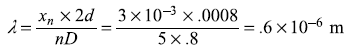
Two slits are placed 0.8 mm apart and the fringes are observed on a screen 0.8 m away from the slit system. With a monochromatic source of light of wavelength λ, it is found that the fifth bright fringe is situated at a distance of 3.0 mm from the central fringe. What is the value of λ?

Exercise 2.4

What is the longest wavelength of X-rays that can be analysed by a rock salt crystal of spacing d = 2.84 Å in the first order?

Exercise 2.5

The distance between adjacent planes in a crystal is 3.2 Å. What is the smallest angle of Bragg scattering for X-rays of wavelength 0.32 Å?

Exercise 2.6

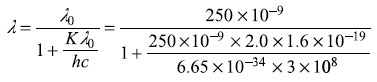
The maximum wavelength of radiation for photoelectric emission in a metal is 250 nm. In order to get photoelectrons from this metal with a maximum kinetic energy of 2.0 eV, what wavelength of radiation must be used?

Exercise 2.7

Explain that it is not possible for a free electron to absorb all the energy and linear momentum of a photon incident on it.

Exercise 2.8

An X-ray photon of wavelength 0.1 nm collides with an electron and is scattered through 90°. What is its new wavelength?

Exercise 2.9

In a Compton scattering experiment, a photon of frequency ν is scattered by an electron which is at rest initially. What is the maximum possible kinetic energy of the recoil electron?

SOLUTIONS

Solution 2.1

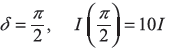
The resultant intensity at points where the waves from the two sources superpose with phase difference δ is

 

where I₁ and I₂ are the intensities of individual waves.

•  
  
•  
  
•  
  
•  
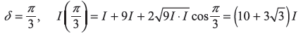
  δ = π,         I(π) = 4I

Solution 2.2

For maxima, the path difference Δ between the two rays originating from two coherent sources must be integer multiple of λ. That is

 

 

Therefore, if at a point (on the screen) one observes n₁th order maxima for light source of wavelength λ₁ and n₂th order maxima for light of wavelength λ₂, then

 

or

Here,

 

Therefore, the 12th order maxima can be observed.

Solution 2.3

The distance of nth bright fringe x_n from the centre of the central fringe is given by

Therefore,

Solution 2.4

Following Bragg’s equation

 

 

∴

Solution 2.5

 

Solution 2.6

The maximum kinetic energy K of photoelectron is given by

or

Solution 2.7

(A) Non-relativistic treatment:

If a photon is absorbed by a free electron at rest, then conservation v of energy and linear momentum dictates,

From these two equations, we get

which is not possible.

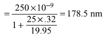
(B) Relativistic treatment:

or

 

 

Equations (2.27a) and (2.27b) cannot be satisfied simultaneously.

Hence, it is not possible for a free electron to absorb a photon. That is why the photoelectric effect takes place under the condition that the incident photons strikes electrons bound in the metal.

Solution 2.8

 

Hence new wavelength is

 

Solution 2.9

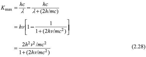
From energy conservation, the kinetic energy K of the recoil electron is

where

K is maximum when λ′ is maximum, that is, when

Therefore,

REFERENCES

1. Beiser, A. 2003. Concepts of Modern Physics, 6th edn. McGraw-Hill.
2. Bohm, D. 1951. Quantum Theory. New York: Prentice Hall.
3. de Espagnat, B. 1976. Conceptual Foundations of Quantum Mechanics. 2nd edn. Reading, MA: Benjamin.
4. Fenynman, R.P., Leighton, R.B. and Sands, M. 1965. The Feymnan Lectures on Physics, volume III, MA: Addison-Wesley.
5. Jammer, Max. 1966. The Conceptual Development of Quantum Mechanics. New York: McGraw-Hill.
6. Deepak Kumar, and Ishwar Singh, 1987. ‘Reality in Quantum Mechanics’, Physics Education 3, 34.
7. Mermin, N.D. 1985. ‘Is the Moon There When Nobody Looks? Reality and the Quantum Theory’, Physics Today, 38, 38.
8. Omnes, R. 1994. The Interpretation of Quantum Mechanics. Princeton, NJ: Princeton University Press.
9. Ishwar Singh, and Whitaker, M.A.B. 1982. ‘Role of the Observer in Quantum Mechanics and the Zeno Paradox’, Am. J. Phys. 50, 882.