Chapter 6

The Linear Harmonic Oscillator

6.1   INTRODUCTION

In the previous chapter, we solved one-dimensional Schrodinger equation of a particle in simple potentials like potential well, step potential, rectangular potential barrier, and so on. In this chapter, we continue to solve Schrodinger equation; this time in a one-dimensional harmonic potential A particle put in this potential is under the influence of central force given by

Here k is termed as the force constant. The quantum mechanical study of one-dimensional harmonic oscillator is very useful as it helps in understanding problems such as vibrations of individual atoms or ions in molecules and solids. In the next section, we briefly review the dynamics of a classical harmonic oscillator.

6.2   CLASSICAL HARMONIC OSCILLATOR

The classical equation of motion of a particle of mass m put in a harmonic potential (e.g. mass m attached with an ideal spring of force constant k) is given by Hooke’s law

In terms of the angular frequency ω, given by

Equation (6.2) appears as

Its solution may be written as

 

 

where x_o is the amplitude of the simple harmonic motion.

Total energy of the particle is (denoting (dx/dt) by ẋ)

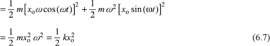
The kinetic energy T of the particle is

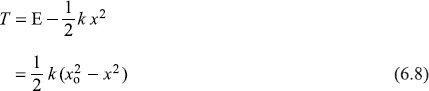
when x = ±x_o, particle comes to rest. Such points are called turning points. The regions are totally forbidden classically, as here the kinetic energy T is negative.

At this stage, let us calculate the classical probability density P_cl(x). By the definition of probability density P_cl(x) dx is the probability of finding the particle in the interval between x and x + dx. If we look at the oscillating particle between –x_o and x_o, we notice, the particle passes the region around x = 0 very quickly and becomes very slow while reaching x = ±x_o. Thus particle spends less time in the central region and more time near turning points regions. Naturally, the probability of particle being found in the central region is small and is large towards the turning points regions. We shall see below, mathematically, the expression of P_cl(x) has this said feature.

Let T_o denote the time period of oscillation of the particle.

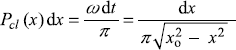
Now P_cl(x)dx, the probability of finding the particle in the interval x and x + dx is [dt/(T_o/2)], where dt is the time interval during which the particle remains in the said length interval dx. That is,

Now

From Eq. (6.5)

so

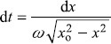
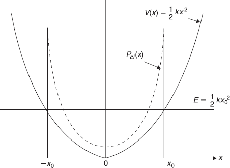
Figure 6.1 Plot of harmonic potential V(x) (solid curve). Also shown is the plot of classical probability density P_cl (x) (dashed curve) for a particle with total energy

Therefore,

and

In Figure 6.1 we have shown the plot of classical probability density P_cl(x).

6.3   QUANTUM HARMONIC OSCILLATOR

Let us now turn to the quantum mechanical description of the harmonic oscillator. Obviously we shall start with the corresponding Schrodinger equation. The Hamiltonian of a particle of mass m put in one-dimensional harmonic potential is

The corresponding time-independent Schrodinger equation is

or

In this chapter, we solve this equation by the so-called series method. In Chapter 8, we shall discuss its solution by the method using raising and lowering operators (also called as creation and annihilation operators).

To solve Eq. (6.16), let us introduce the dimensionless variable

Equation (6.16) may be written in terms of new variable ξ. We have

and

Using these relations, it can be easily seen that Eq. (6.16) becomes

where

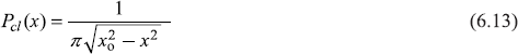
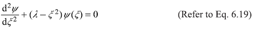
Let us firstly see the asymptotic behaviour of ψ(ξ), that is, the behaviour of ψ(ξ) for |ξ| → ∞. For very large value of ξ the quantity λ appearing in Eq. (6.19), corresponding to finite values of total energy E, may be neglected in comparison to ξ². So Eq. (6.19) reduces to

It can be easily seen that for large values of |ξ|², the functions

satisfy the Eq. (6.21).

From Eq. (6.22)

In Eq. (6.22), the exponent must contain only the minus sign, otherwise the wave function shall diverge for ξ → ±∞, which is unacceptable. The asymptotic form of the wave function, Eq. (6.22) with –ve sign in the exponent, suggests the following form of the solution to Eq. (6.19)

where H(ξ) is some function of ξ, reducing to ξ^p in asymptotic limit. Now we proceed to find the form of function H(ξ). It is a very simple exercise to see that Schrodinger equation [Eq. (6.19)], with Eq. (6.25) becomes

This equation is called as Hermite equation. Let us solve this equation by expanding H(ξ) in a power series in ξ. The harmonic potential has the symmetry V(–x) = V(x). Therefore, the wave functions of the corresponding Schrodinger equation [Eq. (6.16)] must have a definite parity [see Section (6.6)]; the wave function is either symmetric or antisymmetric in x (or in ξ). Let us firstly consider the symmetric eigenstates.

6.3.1   Symmetric Eigenstates (Even Parity States)

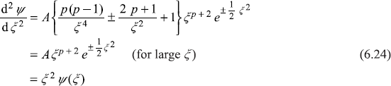
The power series for the symmetric wave function H(ξ) [for which H(–ξ) = H(ξ)] may be written as

Substituting Eq. (6.27) in Eq. (6.26), we get

The first term gives

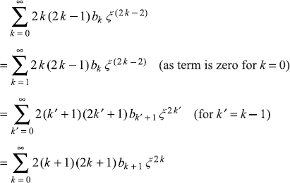
So Eq. (6.28) becomes

Since Eq. (6.29) is valid for all values of ξ, the coefficient of each power of ξ separately, should be equal to zero; giving the recursion relation

Using above equation, values of all coefficients b_k appearing in Eq. (6.27) for H(ξ) may be determined successively in terms of b_o(b_o ≠ 0). Thus an even solution H(ξ), in the form of a series, has been obtained. Let us now analyse a situation when the series does not terminate. In that case, for very large values of k, Eq. (6.30a) gives

If we consider a function ϕ(ξ) = e^ξ2, its series expansion is

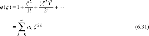
where coefficient a_k = (1/k!). The ratio of two consecutive coefficients is

The ratio in Eq. (6.32) is same as that in Eq. (6.30b). Therefore, if the series [Eq. (6.27)] for H(ξ) does not terminate, the asymptotic form of H(ξ) is similar to that of e^ξ2. Putting this in Eq. (6.25), the wave function ψ(ξ) is seen to have asymptotic behaviour like

or

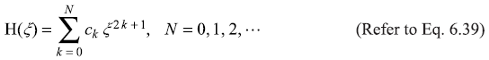
which is not allowed, as it diverges for |ξ|→ ∞. This divergence may be avoided if the series [Eq. (6.25)] terminates at some stage. Let the highest power of ξ² in the resulting polynomial be ξ^2N, where N = 0, 1, 2, 3,···. So Eq. (6.27) becomes

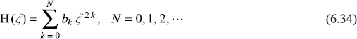
Here coefficient b_N ≠ 0 while coefficient b_{N + 1} is zero. This condition dictates [from recursion relation (6.30a)] that λ has only discrete values given by

 

6.3.2   Antisymmetric Eigenstates (Odd Parity States)

The power series for the antisymmetric wave function H(ξ) for which H(–ξ) = –H(ξ) may be written as

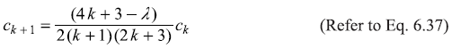
Just like the symmetric case, it can be easily checked that when Eq. (6.36) is substituted in Eq. (6.26), we get the recursion relation

For large values of k, the above equation gives

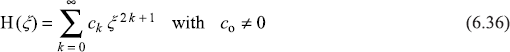
Therefore, just like the previous case, the wave function ψ(ξ) given by Eq. (6.25) will diverge provided the series in Eq. (6.36) terminates at some stage. Let the highest power of ξ in the resulting polynomial be ξ^2N+1, where N = 0, 1, 2, ... Eq. (6.36) then becomes

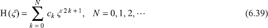
Here c_N ≠ 0, while c_N+1 = 0. This condition, when used in recursion relation [Eq. (6.37)], makes λ to have discrete values given by

 

6.3.3   Discrete Energy Levels

Allowed values of λ from Eqs (6.35) and (6.40) are

and

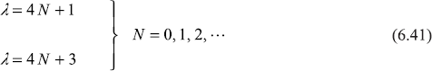
For different values of N = 0, 1, 2, 3, ..., these two equations give respectively the following value of λ

 

or

and

or

So all allowed values of λ, put together, are

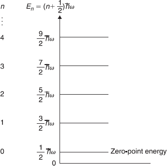
Figure 6.2 Equi-spaced energy levels of a one-dimensional harmonic oscillator. Lowest energy of harmonic oscillator (called as ‘zero-point energy’) is

or 

 

With these allowed values of λ, Eq. (6.20) gives allowed values of energy, E_n as

It may be noted here that whereas the energy E of a classical harmonic oscillator can have any value, the allowed energy values [given by Eq. (6.43)] of a quantum harmonic oscillator are and so on (see Figure 6.2).

6.4   THE NORMALIZED WAVE FUNCTIONS

6.4.1   Even Parity Wave Functions

The Eq. (6.34) gives even parity function H(ξ) as

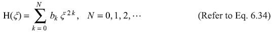
where b_k’s are given by the recursion relation

It may be noted that here λ has allowed values 1, 5, 9, 13, and so on, as λ is given by Eq. (6.35).

 

Using relation (6.30), it can be easily seen that

1. For λ = 1, k = 0, b₁ = 0        (6.44a)
2. For λ = 5, k = 0, b₁ = –2b_o        (6.44b)
3.  
   
4.  
   

From these values, we can write the form of first four even parity functions H(ξ).

 

For λ = 1,   H_o(ξ) = b_o        (6.45a)

 

For λ = 5,   H₂(ξ) = b_o – 2b_oξ²         (6.45b)

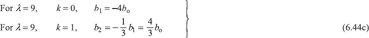
For λ = 9,   H₄(ξ) = b_o– 4b_oξ² + b_oξ⁴         (6.45b)

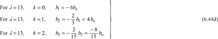
For λ = 13,   H₆(ξ) = b_o – 6b_oξ² – b_oξ⁶        (6.45b)

6.4.2   Odd Parity Wave Functions

Odd parity functions H(ξ) are

where c_k’s are given by the recursion relation

Allowed values of λ here are

 

So using Eq. (6.37), we get

1. For λ = 3, k = 0, c₁ = 0        (6.46a)
2. For λ = 7, k = 0,         (6.46b)
3.  
   

Form of first three odd parity functions H(ξ) are

For λ = 3,    H₁ (ξ) = c_o ξ        (6.47a)

For λ = 7,            (6.47b)

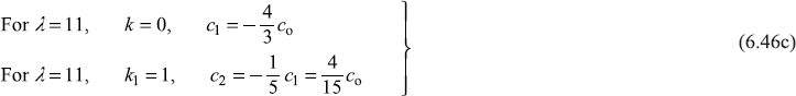
For λ = 11,           (6.47c)

Putting expressions of H(ξ) from Eqs (6.45) and (6.47) in Eq. (6.25), we get the expressions of first few (un-normalized) eigenfunctions

These wave functions, when normalized using the value of definite integral can be written as

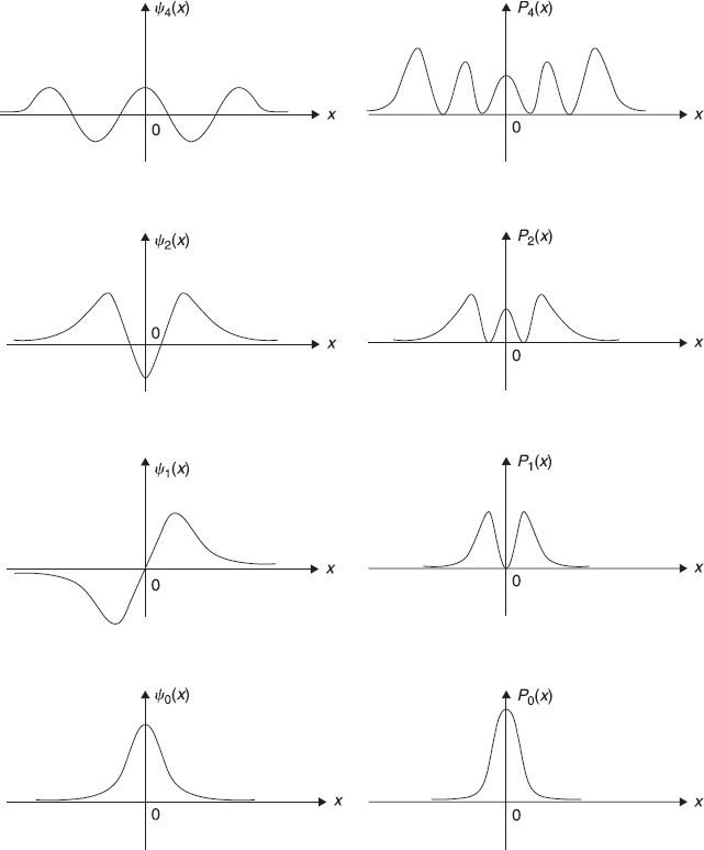
Figure 6.3 The first few eigenstates ψ_n(x) of a one-dimensional harmonic oscillator and the corresponding probability densities P_n(x)

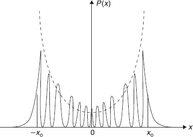
Figure 6.4 Schematic plot of classical probability density (dashed curve) and quantum mechanical probability density (solid curve) for large quantum number

It may be easily checked that the wave functions of harmonic oscillator satisfy the condition of orthonormality

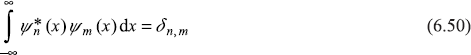
where δ_{n, m} is the Kronecker delta-function.

In Figure 6.3, we show schematic plot of wave functions ψ_o(x), ψ₁(x), ψ₂(x), ψ₄(x) and the corresponding probability densities P_o(x), P₁(x), and so on. In Figure 6.4, we show the probability density P_n(x) for relatively large value of n. We observe that P_n(x) undergoes rapid oscillations as a function of x and its average value is in qualitative agreement with that of the classical probability density. And, in fact, larger the value of n better will be the agreement with classical case. This is nothing but Bohr correspondence principle, which states that the results of quantum theory must approach asymptotically to those obtained from classical theory in the limit of very large quantum numbers (See Appendix A.3).

6.5   THE HERMITE POLYNOMIALS

Let us now return to the Schrodinger equation for harmonic oscillator.

With the substitution

and realizing the fact that for both the even and odd cases, the solutions of Eq. (6.19), corresponding to the eigenvalues of

 

 

are given by

the polynomials H_n(ξ) (called as Hermite polynomials) satisfy the Hermite equation.

The properties of Hermite polynomials H_n(ξ), which are the solutions of Hermite equation [Eq. (6.52)] may be found in a number of text books on mathematical physics. As solving Eq. (6.52) is only an alternative way of getting the form of eigenfunctions ψ_n(ξ) [one way we have already discussed in Sections 6.3 and 6.4 for getting H_n(ξ)], we only mention some of the properties of Hermite polynomials:

The Hermite polynomials may be generated by any one of the functions

and Hermite polynomials satisfy the recursion relations.

 

 

and

Putting the form of Eq. (6.53b) of H_n(ξ) in Eq. (6.51), the nth eigenstate ψ_n(ξ) may be expressed by the formula

Using Eqs (6.53) some of the Hermite polynomials may be obtained as

 

 

 

 

 

 

 

When these expressions of Hermite polynomials are used in Eq. (6.51) and wave functions ψ_n(ξ) are normalized, we find the same expressions of ψ_n(ξ) as given above in Eqs (6.49).

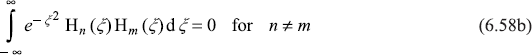
The orthonormality of Hermite polynomials is given as

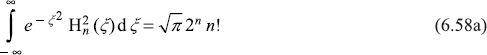
and

6.6   PARITY

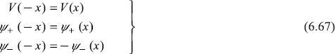
Let us discuss some general features of the solutions ψ(x) [Eq. (6.16)] as a consequence of the symmetry of the harmonic potential V(x) = (1/2) kx². The potential is an even function of x,

 

Let us replace x by –x in Eq. (6.15). We get

or

So as a consequence of the symmetry of V(x) we find that if ψ(x) is an eigenstate, then the function ψ(–x) is also an eigenstate (with the same energy eigenvalue E). There may be two different cases of non-degenerate states and degenerate states. Let us discuss these separately.

6.6.1   Case I: Non-degenerate States

In this case, there is only one eigenstate corresponding to the energy eigenvalue E. Therefore, the two eigenfunctions must be linearly dependent, that is, there must exist a number A such that

 

If the transformation x → –x is made once more in Eq. (6.61), we get

 

 

Hence A² = 1, so that A = ± 1 and we get

 

 

which shows that an eigenstate ψ(x) in a symmetric potential V(x) is either an even or an odd function of x. In other words, ψ(x) has a definite parity; if ψ(–x) = ψ(x), the parity of ψ(x) is even, if ψ(–x) = –ψ(x), the parity is odd.

6.6.2   Case II: Degenerate States

In this case, there are more than one linearly independent eigenstates corresponding to energy eigenvalue E. This happens quite often in two- and three-dimensional systems, for example, two- and three-dimensional (isotropic) harmonic oscillator. These degenerate eigenstates need not have a definite parity. But it is always possible to have linear combinations of these eigenstates such that each state so formed may have a definite parity. For example, let us assume that one of the states ψ(x), corresponding to energy E, does not have a definite parity. Then we may write

 

where

has even parity, and

has odd parity. Putting Eq. (6.64) in the Schrodinger equation [Eq. (6.15)], we have

Now, let us change x to –x in the above equation and noting that

We find

Let us add and subtract Eqs (6.66) and (6.68) to get,

and

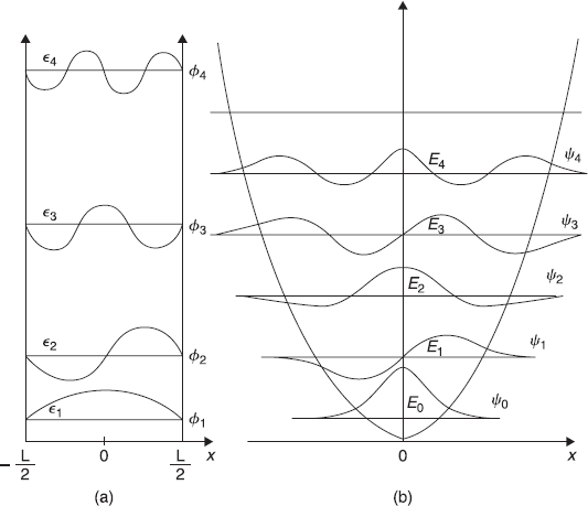
Figure 6.5 Schematic plot of a few wave functions of a particle (a) in one-dimensional potential box of width L and (b) in a one-dimensional harmonic potential

Hence, we notice that ψ₊(x) and ψ_(x) are separate solutions of the Schrodinger equation [Eq. (6.15)], corresponding to the same energy eigenvalue E.

Thus for both the non-degenerate as well as the degenerate cases, every eigenfunction in a symmetric potential can always be chosen to have definite parity.

6.7   CONCLUSIONS

Let us conclude this chapter by comparing the wave functions of a particle in one-dimensional harmonic potential with those of a particle in a one-dimensional potential box. In Figure 6.5, we show first few wave functions, side by side, for both the potentials. In Figure 6.5(a), wave functions are denoted by ϕ₁, ϕ₂, ϕ₃, ϕ₄ (with corresponding energies as ∊₁, ∊₂, ∊₃, ∊₄). The two ground state wave functions ϕ₁ and ψ_o look alike in the middle (i.e., around x = 0). Both the wave functions decrease as | x | increases. But the wave functions ϕ₁, decreases to zero at x = ± (L/2), whereas the wave function ψ_o decreases only exponentially (near the classical turning point) and is non-zero even beyond the classical turning point. If we compare next higher energy wave functions (ϕ₂ and ψ₁), these are again similar in the middle region. Both are having a node at x = 0 and maxima in |ϕ₂| or |ψ₁| on either side. [The points in coordinate space (in the present context it is one-dimensional space so points on x- axis) at which the wave function has value zero, are called nodes of the wave function]. In fact, if we forget about the nodes in ϕ_n at the boundaries [x = – (L/2) and x = (L/2)], the number of nodes appearing in each of the wave functions ϕ_n+1 and ψ_n are n. The energy eigenvalue of a state increases as its number of nodes increases. A similar situation happens for the frequency of classical vibrating string clamped at its both ends. In this case, the frequency of vibrations v of the string increases as the number of nodes n in the string increases.

EXERCISES

Exercise 6.1

A small ball of mass 0.1 mg is attached to a spring of spring constant k = 10^–4 kg s^–2. This ball passes through the equilibrium position with a velocity of 1 m/s.

• Find out the classical amplitude of oscillations.
• Estimate the quanta of energy hω of this oscillator.
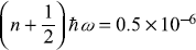
• Estimate the quantum number associated with the energy of the particle.
• Estimate the average spacing between zeros of the eigenstate with such a quantum number.

Exercise 6.2

Start with a trial wave function for the ground state of one-dimensional harmonic oscillator ψ_o(x) = Ae^–bx2n, where b is a positive constant and n is positive integer. Show that the only permissible solution corresponds to n = 1.

Exercise 6.3

Consider a harmonic oscillator in a state described by the wave function

ψ(x, 0) = A[ψ_o (x) – ψ₁(x)], where ψ_o (x) and ψ₁ (x) are normalized eigenstates.

•  Find the normalization constant A.
• Find ψ (x, t)
• At what time t the wave function ψ (x, t) shall be orthogonal to the initial wave function ψ (x, 0)?

Exercise 6.4

Show that Hermite polynomials H_n(ξ) generated by Eqs (6.53a) and (6.53b) are equivalent.

SOLUTIONS

Solution 6.1

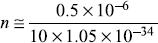
• Total energy = mv² = × 10^–6 × 1 = 0.5 × 10^–6 J

  If A is the amplitude of oscillations, then

  total energy = k A² = 0.5 × 10^–6 J

  so,

  
•  
  
  ħω = 1.05 × 10^–34 × 10 ≃ 10^–33 J
•  
  

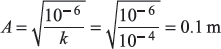
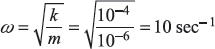
  so,

  
  ≈ 10²⁷

   

• n is the number of nodes in state ψ_n (within classical turning points)

  ∴

  spacing between nodes ≈ ≈ 10^–28 m

 

Solution 6.2

We have

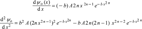
Substituting the trial wave function ψ_o(x) in the Schrodinger equation

we get

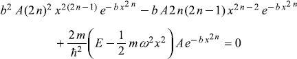
or

For this equation, to hold good (for all values of x), coefficients of all powers of x should be zero. The only possible solution seems for n = 1, for which this equation gives

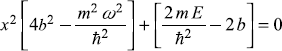
Equating coefficients to zero

and

So

Solution 6.3

• Normalization of ψ(x, 0) gives

   

  1= A²(1 + 1)

  So

  
•  
  
•  
  

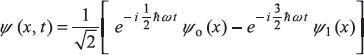
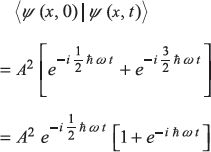
  If ψ (x, t) is orthogonal to ψ (x, 0), then

  

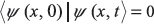
  So

   e^–iħωt = –1

  or

   ħωt = n

  or

  

REFERENCES

1. Gasiorowicz, S. 1996. Quantum Physics. 2nd edn., New York, NY: John Wiley & Sons.
2. Bohm, D. 1989. Quantum Theory. New York, NY: Dover Publishers.
3. Griffith, D. 1995. Introduction to Quantum Mechanics. Englewood Cliffs, NY: Prentice Hall.
4. Powell, J. and B. Crasemann, L. 1961. Quantum Mechanics. Reading, MA.: Addison-Wesley.
5. Liboff, R.L. 1992. Introductory Quantum Mechanics. Reading, MA.: Addison-Wesley.