Appendix C
Some Mathematical Relations
C.1 SOME ALGEBRAIC RELATIONS
C.1.1 Expansions
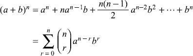
Here the binomial co-efficient 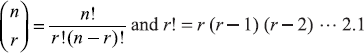 is called ‘factorial r’.
C.1.2 Factors
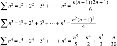
C.1.3 Sum of Numbers
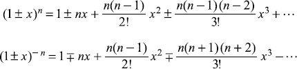
C.1.4 Binomial Series for x2 < 1
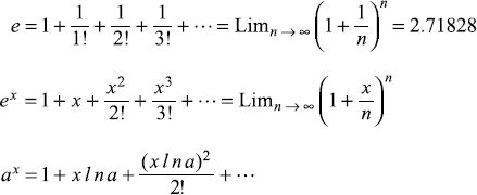
C.1.5 Exponential Series
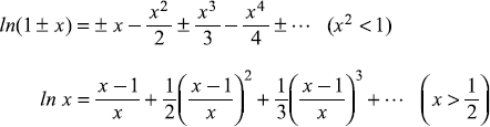
C.1.6 Logarithmic Series
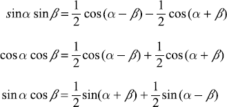
C.2 SOME TRIGONOMETRIC RELATIONS
C.2.1 Fundamental Identities
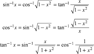
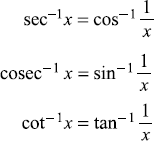
C.2.2 Relations among Inverse Functions
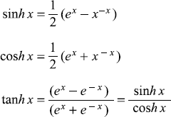
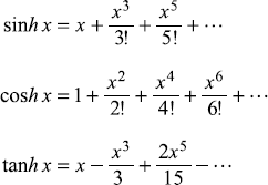
C.2.3 Hyperbolic Functions
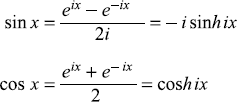
C.2.4 Connection between Circular and Hyperbolic Functions
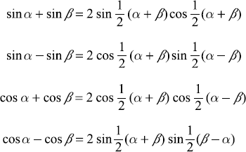
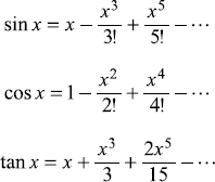
C.2.5 Trigonometric Series
C.3 COORDINATE SYSTEMS
- Cartesian Coordinate System

Figure C.1 Cartesian coordinate system. The differential volume is dV = dx dy dz
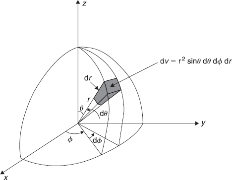
- Spherical Coordinate System
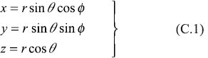
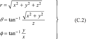
Figure C.2 Spherical coordinate system. The differential volume is dV = r2 sin θ dr dθ dϕ
Unit vectors ex, ey, ez in cartesian coordinate system and er, eθ, eϕ in spherical coordinate system are related as
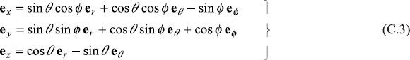
or
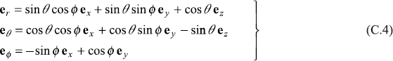
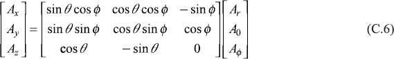
The components of vector A = (Ax, Ay, Az) and A = (Ar, Aθ, Aϕ) are related through the transformation
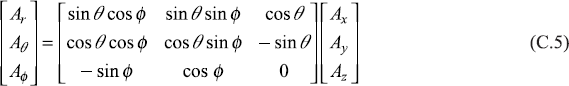
or through inverse transformation
C.4 SOME VECTOR RELATIONS
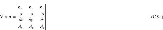
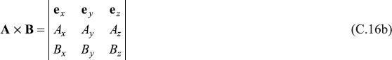
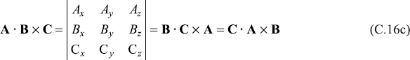
C.4.1 Cartesian Coordinates (x, y, z)

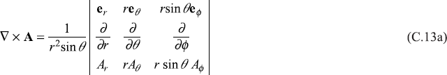
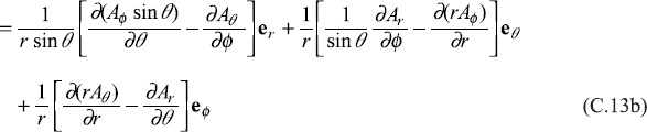
C.4.2 Spherical Polar Coordinates (r, θ, ϕ)
C.4.3 Relations Involving the ∇ Operator
Here A, B, C denote vectors; ϕ, ψ denote scalars.
C.4.4 Other Vector Relations
If r denotes the position vector, then
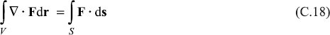
(Gauss) Divergence Theorem: The normal surface integral of a vector function F over the boundary of a closed surface (of arbitrary shape) is equal to the volume integral of the divergence of F taken over the enclosed volume. In mathematical form it is expressed as
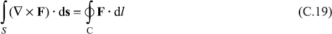
(Stokes) Curl Theorem: If a vector function F and its first derivative are continuous, the line integral of F around a closed curve C is equal to the normal surface integral of Curl F over an open surface bounded by C. In mathematical form it is expressed as
C.5 SOME CALCULUS RELATIONS
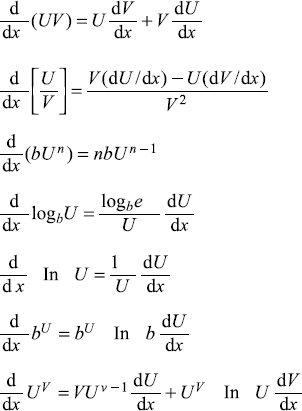
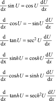
C.5.1 Derivatives
If U = U(x), V = V(x), and b = constant
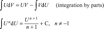
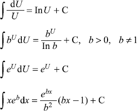
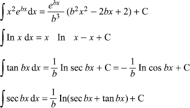
C.5.2 Integrals
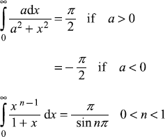
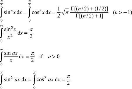
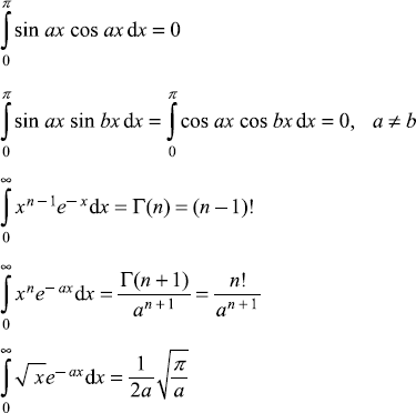
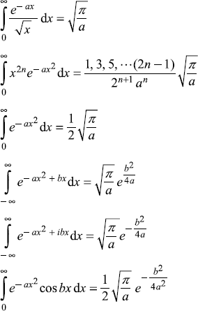
C.6 SOME DEFINITE INTEGRALS
C.7 AN IMPORTANT INTEGRAL
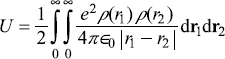
If the electronic charge density in a state in an atom is ρ(r) (e.g. in s-state of an electron), which is spherically symmetric, then the self-potential energy of the charge cloud is
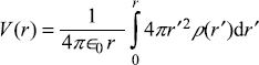
Let us consider the work done in building up this charge distribution. In the process of built up, let us consider that a sphere of charge of radius r is already built. The potential at the surface of this sphere is
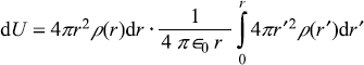
Then the work done in bringing more charge from infinity to form a spherical shell of thickness dr and density ρ(r) at the surface of sphere of radius r already present,
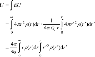
The total self-potential energy for the entire charge distribution is
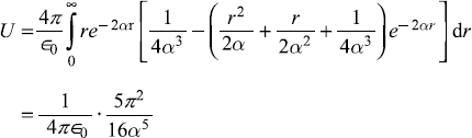
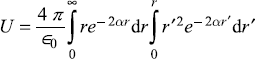
Let us take ρ(r) = e−2αr, so
Integrating by parts, the second integral gives
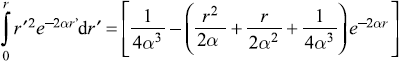
So